Importing GPR-derived data in 3D GIS

Author: Giacomo Landeschi - Last update: 2023-11-20

Introduction

The tutorial shows the users how to import data derived from Ground-Penetrating Radar (GPR) acquisition in a 3D GIS. These datasets typically consist of three-dimensional point clouds defined by vector points associated to the different sampling units recorded by a GPR sensor.

In the context of Ground-Penetrating Radar (GPR) acquisition (for more details on this exploration method, refer to Goodman and Piro, 2013), a key benefit is the ability to gather subsurface information at various depths and generate a data output represented as a three-dimensionally interpreted anomaly. This anomaly is likely to correspond to the archaeological feature under investigation, manifesting either as a void or a "solid" structure. Utilizing specialized software facilitates exporting the interpreted anomaly, presenting it as a singular 3D object in the form of a boundary model and as an ASCII file, which can subsequently be converted into a 3D grid of sampling points. From each XYZ point, vector cubes can be constructed.

Explanation

GPR-derived datasets can provide archaeologists with important information about the extension and depth under the ground surface at which possible archaeological features are located. Despite there is a vast literature pointing out to geophysical methods and GPR in archaeology, it is quite common that these datasets are imported and visualized in GIS as multiple and separate maps, each one featuring an x,y distribution of sensed data at a specific depth under the ground surface of the study area. What is almost missing till now, is a workflow to import and visualize the full three-dimensional GPR dataset in a GIS space. Having such dataset in GIS allows users to make some quantitative analysis on the volumetric data which include a series of Boolean operations including density calculations for instance.

Tutorial

GPR data import follows the following steps:

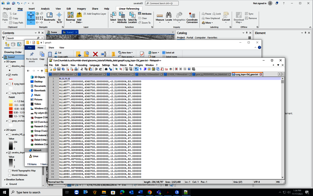
1. Obtain from the specialist in charge of handing the GPR data the acquired dataset in the proper ascii format (.txt, .csv). It is important to make sure that each ascii file presents the point data with x,y,z columns plus a fourth one (g) for the amplitude of the recorded GPS signal.

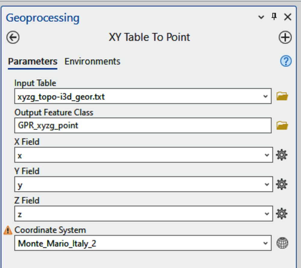
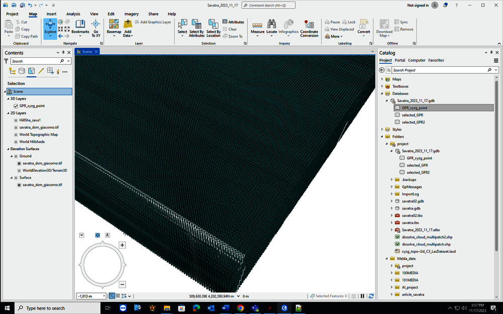
2. In ArcGIS PRO, run the x,y to table function to import the GPR point dataset and visualize it in the correct geolocation.

3. Use the feature class symbology to represent each point as a vector cube and adjust it to the size corresponding to the right sampling units (ex. 0.10 m along x,y coordinates and 0.3 m along z)

4. Export the feature class as a 3D object. This function allows to transform the point shapefile (feature class) into a multipatch feature class, that is the geometrical entity used by ESRI to define 3D objects.

5. Open the new feature class and run the ‘is closed’ function just to double-check thatall the cubes are closed volumes.

6. Run the volume calculation for each cube

How-To

This part contains more detailed instructions on each of the steps described in the tutorial.

1. Open the GPS ascii file with any text editor program (Notepad++ for instance). It si important to make sure that the information is organized in 4 columns with a header line featuring the field values as follows: x,y,z,g. Save the file as a .txt.

2. In ArcGIS PRO, run ‘XY table to point’ function to import the GPR point dataset and visualize it in the correct geolocation. Make sure to correctly assign x,y,z values to the corresponding fields in the table and then define the destination coordinate system.

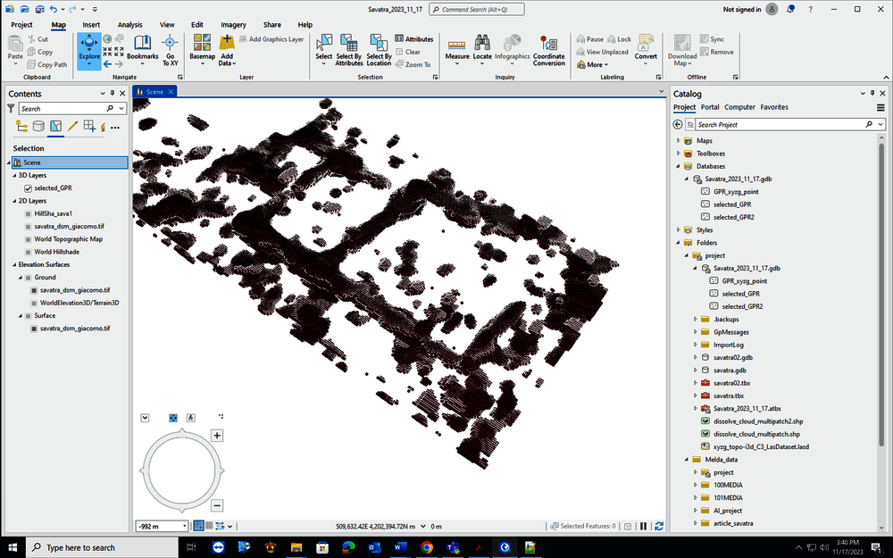
By querying the attribute table, it is possible to select only the range of points with a ‘stronger’ amplitude signal that might correspond to archaeological features:

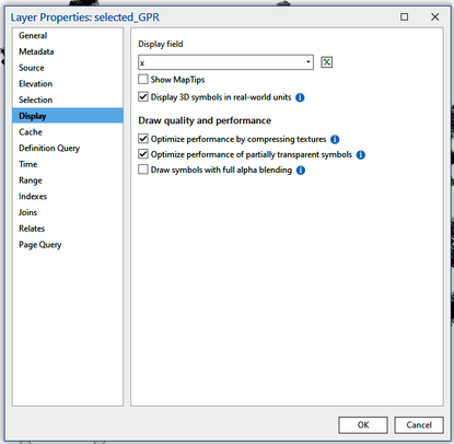
3. Under feature class properties (see below), set the option ‘Display the 3D symbols in real-world units’. This will allow to represent each point with any geometrical object defined according to its right size. The, use the feature class symbology to represent each point as a vector cube and adjust it to the size corresponding to the right sampling units (ex. 0.10 m along x,y coordinates and 0.3 m along z).

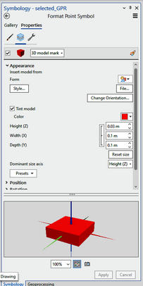
4. Next step of the process is to export the feature class with the adjusted symbology as a 3D object, which will allow to to transform the point feature class into a multipatch feature class.

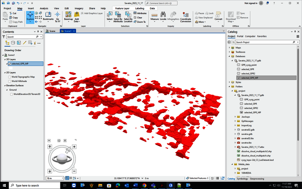
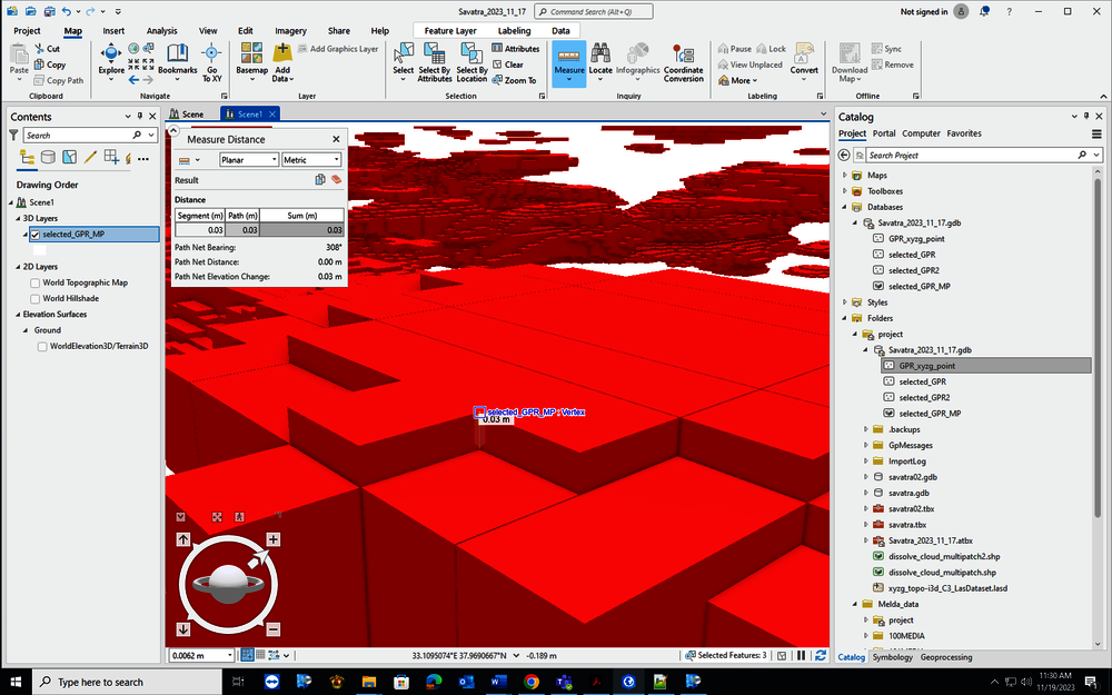
Here, each former amplitude point is represented as a centered vector cube whose size is defined the original sampling interval (in this case, 0.1 m along x,y and 0.03 m along z axes).

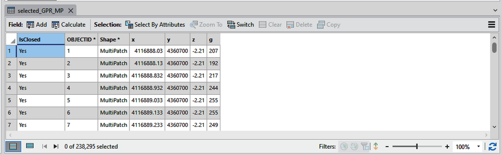
5. Next step is to check that each cube is an enclosed boundary model, for which it is possible to calculate the volume and that can be eventually employed to perform Boolean operations typical of 3D boundary models (intersection, contains, is contained etc.). To do so, search under the ArcGIS toolbox and apply the ‘is closed’ function, which allow users to calculate whether a multipatch feature class is a closed model. If everything is correct, you will see the result of the assessment added as an extra field, ‘is closed’, in the feature class attribute table (see below):

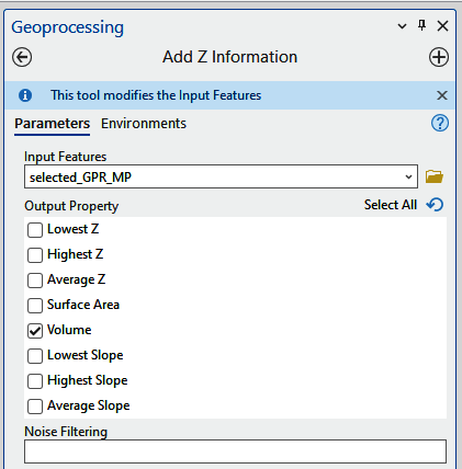
6. To calculate the volume associated to each single cube, use the ‘add Z information’ tool and check the ‘volume’ option (see below). After that a new field will be added to the multipatch feature class attribute table containing