Object-based image analysis
Author: Jan Haas - Last update 2023-10-26
Citation:
Haas, J. (2024). Object-based image analysis (OBIA). Zenodo. https://doi.org/10.5281/zenodo.10687570
Introduction
This tutorial introduces the analyst to Object-Based Image Analysis (OBIA) using ESA Sentinel-1/2 fused data. OBIA involves that pixels are aggregated into groups (segments) with similar spectral or spatial properties. Instead of classifying each pixel individually, the segments are used for classification instead. Apart from image pre-processing and image processing steps alongside accuracy assessment that are described in the tutorials Satellite image processing and Pixel-based supervised image classification, this tutorial focuses on image segmentation and classification. The tutorial is based on remotely sensed data that was created in the tutorial Satellite image processing. After completing this tutorial, the user should be able to derive land use/land cover (LULC) information from satellite data using an OBIA approach. The tutorial is based on straight-forward user-friendly solutions using free and open-source software (QGIS and ORFEO ToolBox).
Tutorial
In order to complete the tutorial, the user will have to install two programs, i.e. QGIS that was used in the previous tutorial Pixel-based supervised image classification and the ORFEO ToolBox that can be used as a plugin within QGIS or as a standalone toolbox.
1. Installing QGIS and the ORFEO ToolBox (OTB)
Image segmentation in QGIS requires the OTB plugin. The toolbox is not installed by default in QGIS. If it is not already installed on your system, the toolbox needs to be installed. If you need to install QGIS, the link to the installer is provided here. Go the the OTB project website and download the appropriate installer for your system and follow the installation instructions. There are two ways to install the OTB. For installation help, it is referred to the following resources:
• How to download and install Ofeo Tool Box (OTB 7.3.0) in QGIS!!
• Add a new plugin repository and Install Orfeo Toolbox in QGis 3
2. Perform image segmentation in QGIS
2.1 Add data to QGIS
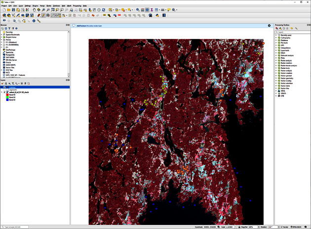
If not already open, open QGIS. Go to Project and save a new template with the name obia_qgis. Go to the Layer tab and choose Add Layer and Add Raster Layer. Add the data that you want to segment, in our case the Sentinel-1/2 satellite image from previous tutorials subset_0_of_S1-S2_stack.tif.
2.2 Segmenting the image
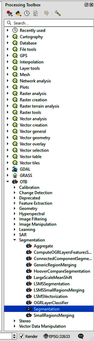
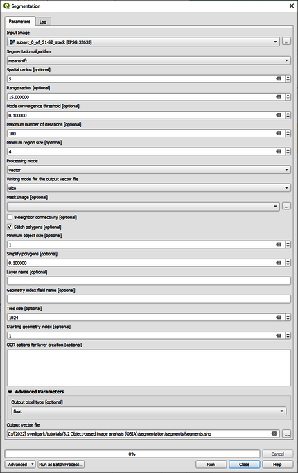
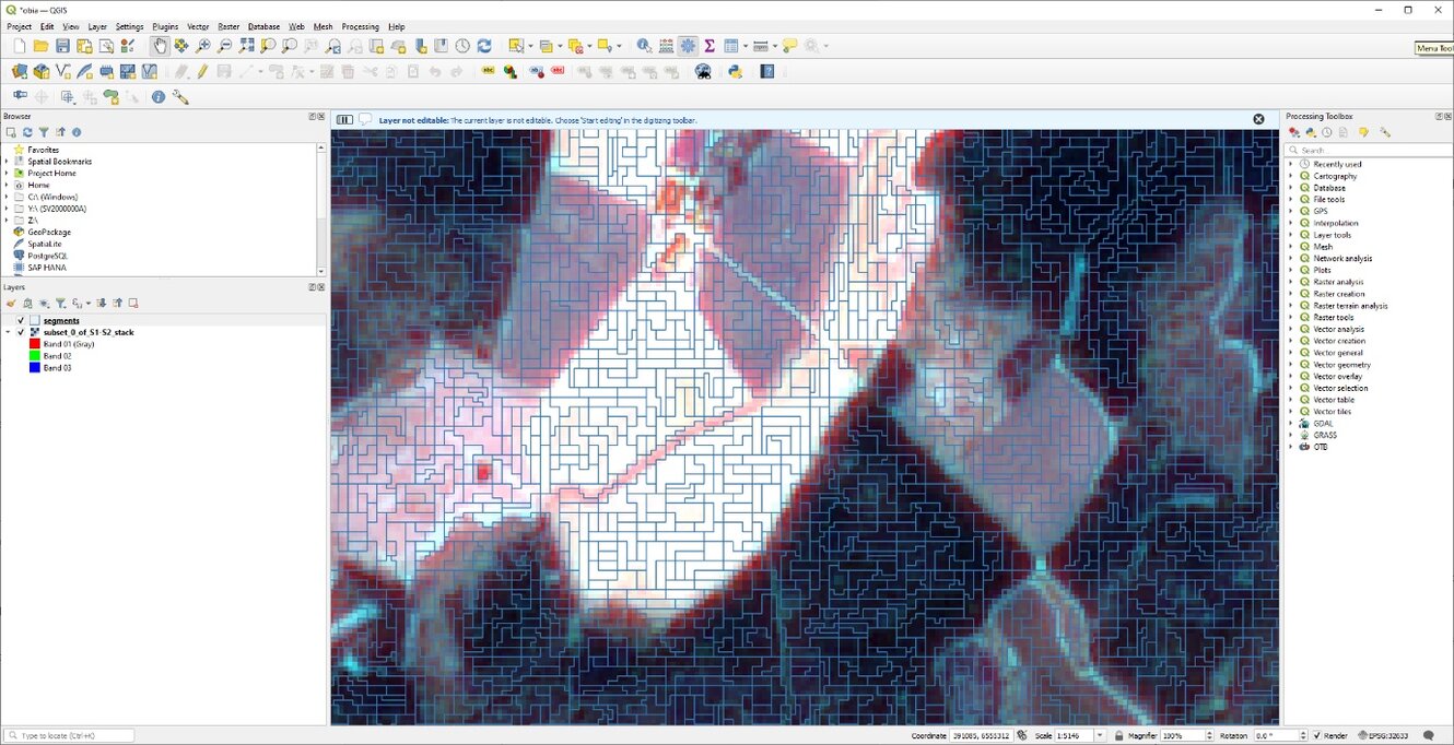
Go to the Processing Toolbox and browse to OTB > Segmentation > Segmentation (Figure 1) and apply the settings as specified in the segmentation dialogue (Figure 2). Read about the segmentation process in the Help section. The minimum region size should be adjusted to the resolution of your data. Start with choosing a value of 4 and adapt after inspecting the segments, i.e., each segment needs to be at least 4 pixels large. Redo the segmentation until the desired segments size is empirically determined. Ideally, no segment should contain more than one desired LULC class. Save the output as segments.shp. Performing the segmentation takes some time (1 hour 59 minutes and 27 seconds) minutes on a Intel(R) Core(TM) i9-10885H CPU @ 2.40GHz; 2.40 GHz mobile workstation with 128 GB RAM and a NVIDIA Quadro RTX 5000 GPU). To decrease computational times, increase the minimum region size. In order to visualize the segments and the original image at the same time, right click on segments.shp and choose Properties. Under the Symbology tab change the fill to Black outline and the stroke width at 0.3 and Apply.
2.3 Create training samples
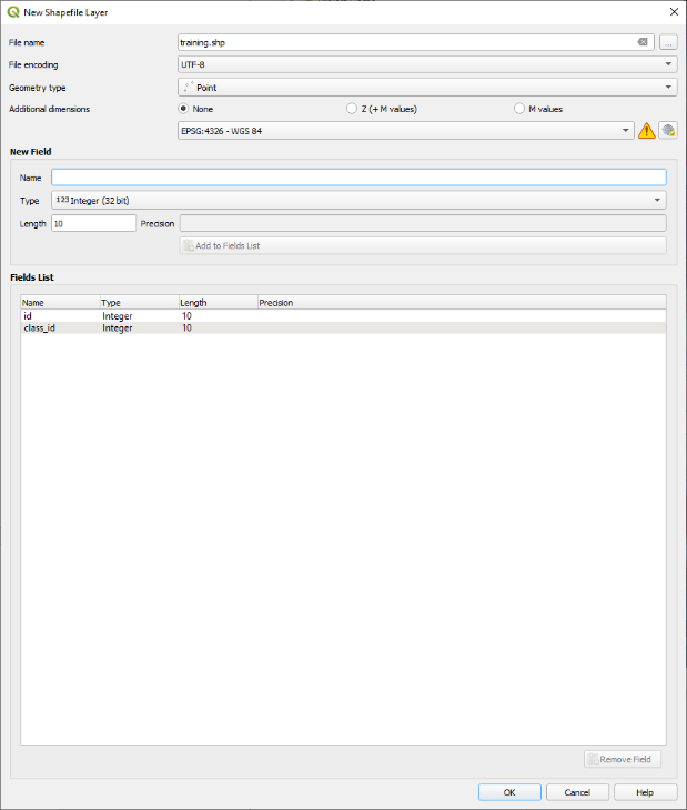
In order to train the classifier correctly we need to create training data from the newly created segments. First, one must define the number desired classes. Go to the Layer tab, choose Create Layer click and New Shapefile Layer. Add the data that you want to segment. Write training.shp as the name of the file, choose the file encoding (UTF-8) and point to the geometry type. Then name the new field class_id and choose type as integer (32 bit) and click on to Add to Fields List (Figure 4).
Create samples for each class in this shapefile by distributing about 30 points over class representative areas. In this tutorial, we create four distinct LULC classes as: 1 Water; 2 Built-up; 3 Forest; 4 Agriculture/Open land. Click on

and then on

to start collecting samples. Define which class will be represented by each feature. Assign a class id from 1 to 4 to each feature (Figure 5).
2.3 Training the classifier
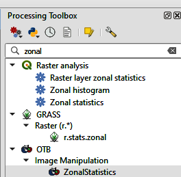
The classifier will extract statistics from the training segments in order to be able to discriminate between the classes. We will use zonal statistics for that. Write Zonal statistics in the Processing Toolbox. Choose OTB > Zonal Statistics (Figure 6).
Select the input image that you are interested in and choose vector as Type of input for zone definitions. Select you segments.shp as input and save the output as segmentation_statistics.shp. Click Run. This process can take a long time. It takes about 12 hours with the settings and computer specifications as described above.
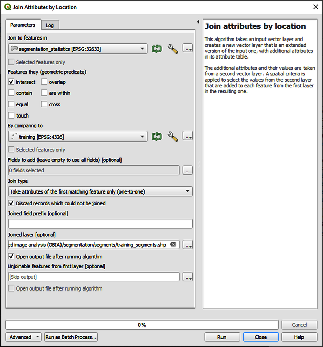
As a next step, we need to transfer the statistics to our training points. This can be done by the Join Attributes by Location function. Write Join to the Processing Toolbox and choose Join attributes by location. Then select segmentation_statistics.shp as Join to features in and training.shp as By comparing to. Choose Take attributes of the first matching feature only (one-to-one) as Join type and check the Discard records which could not be joined box. Figure 7 displays the dialogue. Save the file as training_segments.shp. Click on Run to generate the file.
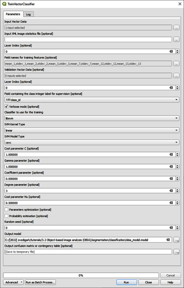
As a next step, we will train the classifier with the extracted statistics from the training segments. Write Train Vector Classifier to the Processing Toolbox. Choose OTB > Train Vector Classifier. As Input Vector Data select training_segments.shp. Right click on training_segments.shp and choose Open Attributes Table in order to check the attributes that have been created i.e.: mean_0, stdev_0, mean_1, stdev1,… up to max13 as we created the statistics for 14 image bands. Depending on the type of image that has been used, you may have a different number of parameters. We will use mean and standard deviation from the original 10 m resolution Sentinel-2 bands as they have the highest spatial resolution and the sigma0 bands from the radar images. Check the boxes for the following Field names for training features [optional]:
mean_1 stdev_1 mean_2 stdev_2 mean_3 stdev_3 mean_7 stdev_7 mean_12 stdev_12 mean_13 stdev_13.
In addition, choose the field that contains the class codes as class_id in the Field containing the class integer label for supervision [optional] list. You may then choose the desired classifier and settings. For this tutorial, keep the classifier as libsvm with default settings and save the output model as obia_model.model as shown in Figure 8.
2.4 Image classification
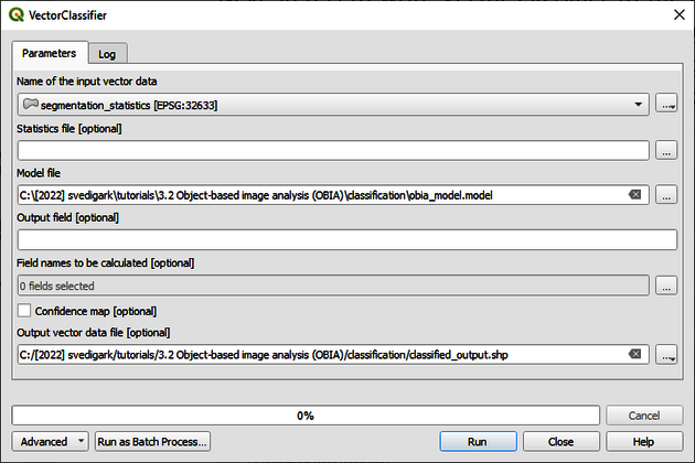
After the classifier has been trained, we can use it to classify the image. Write VectorClassifier in the Processing Toolbox. Choose OTB > Vector Classifier. As input vector data select the segmentation_statistics.shp and choose the obia_model.model as the model file. Check mean_1 stdev_1 mean_2 stdev_2 mean_3 stdev_3 mean_7 stdev_7 mean_12 stdev_12 mean_13 stdev_13 as the field names to be calculated. Save the file as classified.shp (Figure 9). Click on Run.
2.5 Visualize the classification
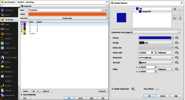
Go to the Layer tab, click on Add Layer and choose Add Vector Layer. Choose classified.shp and click on Add. Right click on classified.shp and choose Properties…. Under Symbology change from Single Symbol to Categorized and choose predicted as the value. Then click Classify. Click on Symbol, Simple Fill and change the Stroke color to Transparent. Click OK twice. The dialogues are shown in Figure 10 below.
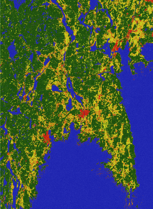
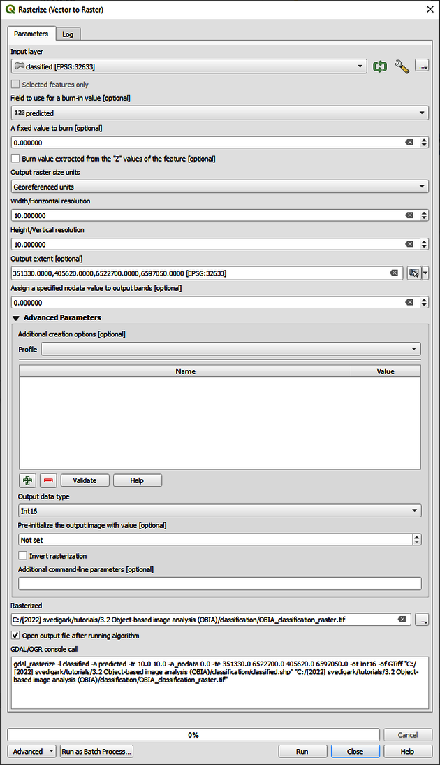
The final classification result is shown in Figure 11 above. If you are satisfied with the classification output, you should now perform accuracy assessment as explained in tutorial Pixel-based supervised image classification. However, as our result is still in vector format, we need to convert it to raster first. Go to Raster > Conversion > Rasterize and enter the parameters as specified in Figure 12 below. Save the output raster file if you want to use it in tutorial Landscape analysis with landscape metrics.
How to
OBIA has become an increasingly significant method within remote sensing applications, particularly in landscape archaeology, as it allows for more precise analysis and understanding of archaeological sites using satellite imagery. Necessary image pre-processing and processing steps prior to OBIA alongside accuracy assessment are described and discussed in the tutorials Satellite image processing and Pixel-based supervised image classification.
General workflow
In this section, emphasis is put on the general workflow alongside segmentation and classification approaches, comprising image acquisition, pre-processing, processing (optional), segmentation, classification and accuracy assessment. The following steps are described in more detail here with respect to landscape archaeology even though the following generic steps should be considered in any OBIA with remotely sensed data.
1. Image acquisition: This is the first step where raw satellite images are acquired for a specific archaeological area of interest. Various freely available multispectral satellite images at medium (Landsat, Sentinel) to very high resolutions like Quickbird or WorldView can be used. The choice of satellite data depends on factors such as spatial resolution, temporal resolution, spectral bands, and cost. In archaeological applications, the area's size, nature of archaeological features expected, and their spatial characteristics play a role in choosing the appropriate satellite data. Image segmentation in remote sensing relies on the inherent variability in the data captured by different sensors. The quality of segmentation depends on factors such as spatial, spectral, and temporal resolution of the data, noise levels, and the sensor's sensitivity to the features of interest.
• Optical Sensors: Multispectral and hyperspectral sensors that capture data in various bands of the visible and infrared spectrum are often the most effective for image segmentation because they provide rich spectral information that can differentiate a wide variety of surface features. Examples include the Landsat series, Sentinel-2, and WorldView. Very high-resolution data can yield more precise segments but may also increase computational demands.
• Synthetic Aperture Radar (SAR): SAR data, which is typically used for applications such as land cover mapping, vegetation monitoring, and disaster assessment, can be difficult to segment due to the speckle noise and complex signal interpretation associated with it. The use of SAR data for segmentation requires specialized techniques, such as despeckling filters and texture features, to yield satisfactory results. In addition, it may be beneficial to integrate SAR data with other types of data in a process called data fusion or multiband combination. For example, combining SAR data with optical data could help mitigate the limitations of SAR and improve the segmentation results. The effectiveness of different sensors and techniques can vary greatly depending on the specific context and goals of your study, so it is always worth experimenting with different approaches to find what works best for one specific use case. SAR data is typically best suited for specific applications rather than for general land cover classification.
• Thermal Sensors: Thermal infrared data can be useful for segmenting features based on temperature differences, such as differentiating between water bodies and land or identifying thermal hotspots. However, because thermal data does not provide as much spectral detail as optical sensors, it might be less effective for segmenting a diverse range of surface features
• LiDAR (Light Detection and Ranging): LiDAR data is useful for segmenting features based on elevation, such as buildings or trees. However, it may be less effective for segmenting features that are not elevation-dependent.
2. Image pre-processing: Once the satellite images are acquired, they need to be pre-processed to be suitable for further analysis. This stage typically involves tasks like radiometric correction (to correct for sensor irregularities and atmospheric conditions), geometric correction (to correct for Earth's curvature, sensor angle, etc.), and image enhancement (to improve the visual interpretability of the image). In archaeological contexts, another critical pre-processing step can be the removal or particular analysis of vegetation cover using spectral indices like NDVI (Normalized Difference Vegetation Index), as this could obscure the underlying archaeological features.
3. Image processing (optional): This step involves further refining the images for specific applications. For instance, image fusion techniques can be used to combine the spatial resolution of one sensor (e.g., Sentinel) with the spectral resolution of another sensor (e.g., Landsat), thereby creating a single image that has both high spatial and spectral detail. This step can be crucial for landscape archaeology, as fusing images from different sensors can highlight various archaeological features that may not be apparent in individual images. Other image processing techniques that are worth considering are Principal Component Analysis (PCA) which is useful for data reduction or texture analysis through Gray Level Co-occurrence Matrix (GLCM) that can improve class separabilities.
4. Segmentation: After the images are appropriately processed, the next step is to segment them. Segmentation in OBIA involves grouping adjacent pixels that share similar spectral properties into homogenous objects or "segments". These segments then represent different features in the landscape (like buildings, roads, fields, etc.) that can be further analysed. The correctness of the segmentation is crucial in landscape archaeology, as poorly defined segments could lead to misinterpretation of archaeological features.
5. Classification: Once the image is segmented, each segment is classified into different classes based on its spectral properties and/or shape and texture attributes. Classification can be performed using various methods, ranging from simple rule-based classifications to complex machine learning models. In the context of landscape archaeology, classes could represent different types of archaeological features or different types of LULC.
6. Accuracy assessment: The final step in the OBIA workflow is to assess classification accuracy. This is usually done by comparing a subset of the classified image with reference data (like ground truth data collected from field surveys or high-resolution aerial images). Accuracy assessment helps determine how well the classification model has performed and identifies areas of improvement for future analysis.
Segmentation
Image segmentation in OBIA is a central step. It involves partitioning an image into multiple segments (sets of pixels, also known as superpixels) where each segment has similar attributes such as colour (digital brightness values) or intensity. The goal is to change the representation of an image into something that is more meaningful and easier to analyse. In the context of landscape archaeology, these segments can represent various features in the landscape, such as ruins, roads, bodies of water, vegetation, and more. When it comes to choosing the right segmentation algorithm, it largely depends on the nature of the image and the specific task at hand. Several algorithms are available, each having its own advantages and disadvantages.
1. Region growing: This method starts with a pixel or group of pixels (seed points) and adds neighbouring pixels that have similar properties.
2. Watershed transformation: This algorithm treats the image it processes like a topographic map, with bright pixels high and dark pixels low.
3. Edge detection: Edge-based methods like Sobel, Prewitt, or Canny algorithms can be useful when the aim is to delineate certain boundaries clearly.
4. Mean-shift and quick shift: These are more sophisticated algorithms that are capable of producing high-quality results, especially for complex images, by mapping the spatial colour distribution of an image and then segmenting the clusters in the mapped space.
When it comes to setting parameters for these algorithms, it is more of an iterative process of trial and error. Some general advice includes:
1. Scale parameter: This controls the size of the objects (segment size) you get. A small scale will yield many small objects, while a large scale will yield fewer, larger objects. In archaeological applications, this should be determined based on the size of the archaeological features you are interested in.
2. Shape and compactness: These parameters control the shape of the segments. If one is trying to delineate linear features, one may want to allow for more elongated segments.
3. Spectral criteria: Some algorithms allow setting a spectral criterion, which can be used to control how much the colour or intensity can vary within a segment. This should be set based on the spectral variability of the features of interest.
Finally, it is worth noting that image segmentation is often an iterative process. One may need to try different algorithms, or different parameter settings within the chosen algorithm, and then assess the results visually or using quantitative measures of segmentation quality before eventually refining the approach based on these assessments.
Classification
Equally important as segmentation, classification is crucial in assigning meaningful LULC to the generated segments based on their spatial and spectral properties alongside other characteristics. There are several classifiers that work particularly well with segmented data in OBIA:
1. Decision Trees: These are rule-based classifiers where each node represents a feature in an instance to be classified and each branch represents a value that the node can assume. Decision trees are easy to interpret and do not require much data pre-processing, but they can be prone to overfitting.
2. Random Forest: Random Forest is an ensemble learning method that operates by constructing a multitude of decision trees during training and outputting the class that is most likely according to majority voting among the individual trees. Random forests correct for decision trees' habit of overfitting to their training set.
3. Support Vector Machines (SVM): SVM is a powerful, flexible, yet easy to understand, supervised machine learning algorithm that can be used for both classification and regression tasks. The goal of the SVM algorithm is to find a hyperplane in an N-dimensional space that distinctly classifies the data points.
4. K-Nearest Neighbors (K-NN): The k-NN algorithm is a non-parametric method used for classification and regression. A sample is classified by a plurality vote of its neighbors, with the object being assigned to the class most common among its k nearest neighbors. It is useful when the decision boundary is very irregular.
5. Neural Networks: These are a set of algorithms modelled loosely after the human brain, designed to recognize patterns. They interpret sensory data through a kind of machine perception, labelling, or clustering raw input. These are powerful tools but can be complex to implement and understand.
6. Naive Bayes: This is a simple probabilistic classifier based on applying Bayes' theorem with strong (naive) independence assumptions between the features. It is fast and simple to understand.
7. Rule-based classification: In this method, a series of rules is constructed to determine the class of a segment. Each rule consists of one or more criteria that use the attributes of the segment (e.g., the mean intensity in a certain spectral band, the segment's shape, etc.). This method allows for high flexibility and the inclusion of expert knowledge, but it can also be time-consuming to set up if the number of classes and attributes is high. When deciding which classifier to use, it is important to consider the nature of the data and task, as well as practical considerations like the complexity of the model, the availability of labelled training data and the computational resources available.
Reference
For references regarding QGIS, image pre-processing, image processing and accuracy assessment please consult the tutorials on Satellite image processing and Pixel-based supervised image classification.
ORFEO ToolBox
The Orfeo ToolBox (OTB) is an open-source project for state-of-the-art remote sensing. Built on the shoulders of the open-source geospatial community, it can process high resolution optical, multispectral and radar images at the terabyte scale. It can be used as a standalone toolbox or be integrated in QGIS.
OBIA
Object-Based Image Analysis (OBIA) is an approach used in geographic image processing that segments an image into distinct objects, or group of pixels, rather than treating individual pixels in isolation. This method is based on the concept that adjacent pixels within an image are likely to belong to the same object and therefore share common features or properties. OBIA begins with image segmentation, which groups pixels into larger, meaningful objects based on some criteria, such as colour or texture similarity. The resulting objects might represent real-world features like buildings, roads, vegetation or water bodies. Once the image is divided into objects, various characteristics of these objects—such as shape, size, texture and spectral information—are analysed. The analysis might involve classifying objects into different categories or detecting changes over time. The main advantage of OBIA over traditional pixel-based analysis is its ability to incorporate spatial and contextual information, making it more closely aligned with human perception and interpretation. This often results in more accurate and detailed analysis, especially for high-resolution images. It is particularly useful in fields like remote sensing, land use analysis, and landscape ecology.
Segmentation
Image segmentation is a critical process in OBIA where an image is partitioned into multiple segments or sets of pixels, often referred to as superpixels. These segments correspond to different objects or parts of objects in the image. The aim of segmentation is to simplify or change the representation of an image into something more meaningful and easier to analyse. Segmentation algorithms generally aim to group together pixels that share similar attributes such as colour, intensity, or texture. The output, often called a segmentation map, serves as the foundation for further object-based image processing tasks like feature extraction, classification, and analysis.
Support Vector Machine (SVM)
A SVM is a supervised learning method used for classification and regression analysis. It works by mapping input data into a high-dimensional feature space, and then constructing a hyperplane or a set of hyperplanes in this space, which can be used for classification, regression, or other tasks. The main strength of SVMs is their ability to handle data that is not linearly separable by using kernel functions to map the original data into a higher dimension where a hyperplane can separate the classes. They are effective in high-dimensional spaces, robust against overfitting, and are versatile in modelling diverse sources of data. SVMs are particularly well-suited to problems where the number of dimensions exceeds the number of samples.
Explanation
Recent studies demonstrate the potential of OBIA in landscape archaeological applications. In an early study, Verhagen & Drăguţ (2012) tested the use of OBIA for automated landform delineation and classification using digital elevation models (DEMs). They found that the technique offers significant advantages over traditional cell-based classification approaches, which have been hampered by shortcomings such as the 'salt-and-pepper effect', the tying of the scale of analysis by raster resolution and difficulties in integrating topological relationships into classifications. Importantly it is pointed out that OBIA can be used to produce landform classifications at any desired scale level. However, the real challenge is to find the appropriate scale levels for image segmentation. They concluded that while OBIA is a promising technique for quick and objective delineation of landform, it still requires an improved conceptual framework tailored to the local situation and archaeological questions to better identify and interpret the derived landform objects.
Sevara & Pregesbauer (2014) examined the value of OBIA in detecting archaeological features from high-resolution remote sensing and geophysical prospection datasets. They noted that while OBIA has been used for this purpose in the past, few applications have approached it from a genuinely object-oriented perspective. In response to this, they presented a method of describing selected archaeological features in object-oriented terms, thereby establishing a framework for an attribute-based approach to archaeological object detection.
More recent studies include Davis et al. (2019) who explored the application of OBIA as a tool for studying anthropogenic mounded features like earthen mounds, shell heaps, and shell rings in the American Southeast. The research addresses the issue of undetected archaeological mound features hidden under dense forest canopies that hinder pedestrian surveys and aerial observations. Using publicly available Light Detection and Ranging (LiDAR) data from Beaufort County, South Carolina, the authors utilized OBIA in combination with morphometric classification and statistical template matching, identifying over 160 previously undetected mound features. This improved our knowledge of settlement patterns by providing systematic insights into past landscapes. The study detailed the differences between pixel-based and object-based methods of analysing remote sensing data, highlighting that OBIA is particularly suited to identifying spatially discrete features varying primarily in topographic structure. A multiresolution segmentation and template-matching within their OBIA approach was used in the study to enhance result accuracy. However, Davies et al. (2019) also acknowledged that template-matching could produce false positives, which they tried to minimize using land-use maps and roadway shapefiles. Despite some limitations, such as the exclusion of disturbed mounds and reliance on a comprehensive template of known mound morphologies, the study demonstrated the potential of OBIA in archaeology. The method allowed for the identification of topographic features across an entire county within a week—a task that would take years using traditional pedestrian surveys. The researchers highlighted the adaptability of this method, offering promise in identifying previously undocumented archaeological features and contributing to the protection of important archaeological sites.
The comprehensive review by Davis (2019) describes the application and development of OBIA in the field of archaeology. OBIA has significantly improved the identification of archaeological features using morphometric and spectral parameters. The use of OBIA in archaeology has grown over the past 15 years, starting with attempts to identify large-scale linear structures, like Roman structures. Early studies that used 2D satellite imagery struggled with high rates of false-positive identifications due to the quality of the data used and the variables incorporated. Implementation of more variables and the use of higher-resolution datasets has improved the accuracy of OBIA for archaeological prospection. By the beginning of the 2010s, researchers began incorporating 3D data such as LiDAR, which improved the detection of archaeological features as topographic information could now be included in multiple dimensions. The use of pattern recognition through template matching has also been successful in identifying archaeological structures. However, it is limited by false-positive and false-negative results. The number of variables used in OBIA has increased in recent years, including topographic measurements such as hillshade, slope, and topographic openness. Results indicate a positive correlation between the number of variables used in OBIA procedures and the accuracy of detection. Expert knowledge of the study area is essential for these automated detection methods to work effectively. Although the majority of studies use OBIA to automate the detection of archaeological features, some researchers are using OBIA to protect and monitor sites at risk of destruction, develop comprehensive maps of archaeological activity, and analyse settlement patterns and socio-political organization. Recent applications of OBIA and machine learning have yielded highly accurate results, such as the detection of over 2000 Neolithic burial mounds with minimal false positives and false negatives. The use of hydrological depression algorithms has also been effective in archaeological mound detection. In conclusion, OBIA has shown significant promise for accurate automated prospection in archaeology. However, there is still much untapped potential for its application. Future research should seek to combine automated algorithms with manual analysis for broader data acquisition, in order to better record, preserve, protect, and study our collective human history.
Magnini & Bettineschi (2019) broadly discuss the potential and challenges of OBIA in archaeology as a rapidly emerging method for integrating data processing techniques and GIS approaches, intending to replicate human perception by using (semi)automated image segmentation and classification. However, the lack of a theoretical framework adapted to archaeology's specificities prevents researchers from establishing a common investigation protocol. The article introduces the concept of Diachronic Semantic Models (DhSM) to integrate the long-term evolution of the archaeological landscape into the object-based approach. They also present an assessment of OBIA's limits and potential using case studies, proposing a general workflow of an Archaeological Object-Based Image Analysis (ArchaeOBIA) project. The authors highlight that automation in archaeological photointerpretation is a controversial issue, but it's crucial given the potential to speed up the examination of large data volumes and improve image analysis reproducibility. Despite initial disappointing results, the use of OBIA in archaeology has grown since 2007, with promising applications in various areas, including the identification of small, round archaeological structures and landform delineation and classification. The paper suggests that the incompleteness and dynamic nature of the archaeological record can be addressed by using ontologies based on DhSM. The authors see ArchaeOBIA as an approach that integrates OBIA and result assessment, striking a balance between processing speed and result reliability. They mention that ArchaeOBIA shows promise in dealing with the complexity of the archaeological record and speeding up image analysis and object recognition. Finally, the authors foresee the use of OBIA expanding in archaeology, anticipating that the proposed ArchaeOBIA approach will enhance rule-set interoperability and open up new possibilities for extracting archaeological information from remotely sensed imagery. This progress will hopefully raise the overall accuracy of results as the knowledge and mental models of archaeologists are systematically integrated into DhSM.
With particular respect to open Sentinel-2 data, Agapiou (2020) recently investigated the use of freely available medium resolution satellite images in archaeological research, an area which is currently underutilized due to spatial resolution limitations. The study aims to demonstrate how a combination of Landsat and Sentinel optical sensors can effectively support archaeological research through OBIA. The fusion of Landsat 8 OLI/TIRS Level-2 and Sentinel-2 Level-1C optical images was performed over the archaeological site of "Nea Paphos" in Cyprus, aiming to enhance the spatial resolution of the Landsat image. Various fusion models such as Gram–Schmidt, Brovey, principal component analysis (PCA), and hue-saturation-value (HSV) algorithms were applied and evaluated, with the Gram-Schmidt fusion method and the near-infrared band of Sentinel-2 (band 8) showing optimum results for detecting monuments and buried archaeological remains without major spectral distortion of the original Landsat image. The study also highlights OBIA's potential for archaeological research, given its ability to segment images and extract features, going beyond traditional pixel-based image analysis. While pixel-based analysis of satellite images is well established, further research is needed regarding OBIA analysis for archaeological studies. The paper concludes that the integration of Landsat 8 and Sentinel-2 optical datasets enhances spatial resolution for archaeological research, with the potential to improve object-oriented analysis and increase the detection rate of archaeological proxies. Future work could focus on further exploring the synergistic use of different sensors and enhancing satellite-based archaeological prospection and management.
References
Agapiou, A. (2020). Evaluation of Landsat 8 OLI/TIRS level-2 and Sentinel 2 level-1C fusion techniques intended for image segmentation of archaeological landscapes and proxies. Remote Sensing, 12(3), 579.
Davis, D. S. (2019). Object‐based image analysis: a review of developments and future directions of automated feature detection in landscape archaeology. Archaeological Prospection, 26(2), 155-163.
Davis, D. S., Sanger, M. C., & Lipo, C. P. (2019). Automated mound detection using lidar and object-based image analysis in Beaufort County, South Carolina. Southeastern Archaeology, 38(1), 23-37.
Magnini, L., & Bettineschi, C. (2019). Theory and practice for an object-based approach in archaeological remote sensing. Journal of Archaeological Science, 107, 10-22.
Sevara, C., & Pregesbauer, M. (2014). Archaeological feature classification: An object oriented approach. South-Eastern European Journal of Earth Observation and Geomatics, 3, 139-143.
Verhagen, P., & Drăguţ, L. (2012). Object-based landform delineation and classification from DEMs for archaeological predictive mapping. Journal of Archaeological Science, 39(3), 698-703.