Landscape analysis with landscape metrics
Author: Jan Haas - Last update: 2023-11-15
Citation:
Haas, J. (2024). Landscape analysis with landscape metrics. Zenodo. https://doi.org/10.5281/zenodo.10687588
Introduction
The aim of this tutorial is to familiarize the user with the concept of Landscape Metrics (LM) and their capacity as landscape descriptors in an archaeological context. The tutorial provides a detailed method for applying LM to remote sensing data in archaeological studies using QGIS and Fragstats. It begins with instructions on installing these essential tools and proceeds to guide users through visualizing both classification and original images in QGIS. The tutorial then moves to image filtering in QGIS. This refined data is then imported into Fragstats for in-depth analysis using nine metrics at class and landscape levels. The tutorial exemplifies how the results can be interpreted, helping users understand each metric's significance in an archaeological context. Metrics like the Landscape Patch Index and Edge Density are explained in terms of their utility for understanding distribution density of archaeological sites, settlement patterns, and interactions between land uses in historical settings. Additionally, the tutorial offers a background on the importance of LM in landscape ecology, stressing their role in assessing biodiversity, habitat fragmentation, and human activity impacts. It also touches on the innovative application of these metrics in archaeology, highlighting the potential to significantly enhance understanding of anthropological and historical landscapes. Overall, this tutorial aims to be a resource for archaeologists and researchers, combining practical analytical steps with theoretical insights. It ensures users not only execute the analysis correctly but also comprehend the implications of their findings in archaeological research.
Tutorial
In order to complete the tutorial, the user will have to install two programs, i.e., QGIS that was used in previous tutorials and the Fragstats software.
1. Install the software
If you need to install QGIS, the link to the installer is provided here. Download and install Fragstats 4.2 from this source and acquire the manual.
2. Visualization of original image/classification and image filtering in QGIS
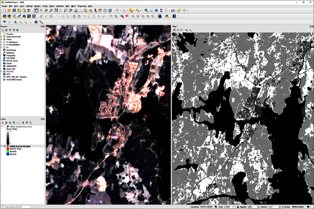
Open QGIS and add the raster image OBIA_classification_raster.tif from the tutorial Object-based image analysis (OBIA) through Layer > Add Layer > Add Raster Layer. Use the same function to additionally add the original image subset_0_of_S1-S2_stack.tif to the project. Synchronize image views through clicking on the View tab > New Map View. Dock the small new window on the screen by dragging and dropping it to the right edge. In the new map window, click the little tool icon (View settings) and check the Synchronize View Center with Main map and the Synchronize scale boxes. In order to visualize the classification in one window and the original image in the other, we need to create new map themes. Make sure that only the OBIA_classification_raster.tif image box is checked in the Layers panel and click on the Manage Map Themes in the Layers box (the little eye icon) and choose Add Theme and call it Classification. Uncheck the classification view and visualize the subset_0_of_S1-S2_stack.tif image instead. Create a new theme and call it Original. In the recently added new map view (Map 1) click the eye icon and choose Classification. The result should look like the one in Figure 1.
3. Image filtering in QGIS
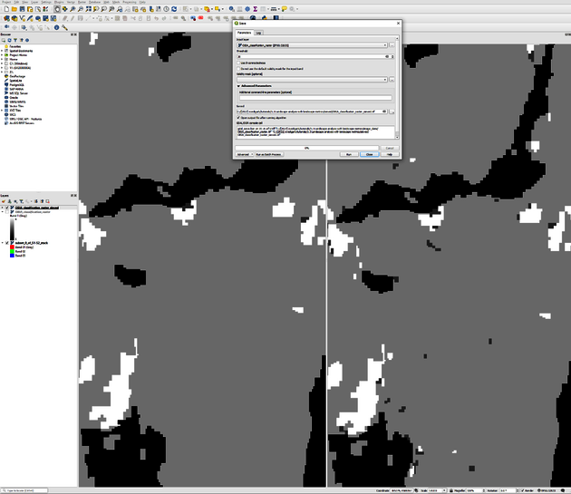
When one is interested in describing the landscape in general without focusing on any particular landscape aspect, small spurious aggregations of pixels that are most likely the result of misclassifications need to be removed. This can be done by the Sieve function. Go to the Raster tab > Analysis > Sieve. Set the Threshold for filtering to 20, i.e., areas smaller than 20 connected pixels of one class will be merged with the surrounding, larger class. Save the output as OBIA_classification_raster_sieved.tif. The result of the Sieve function is displayed in Figure 2 below. Note that smaller unconnected areas have been removed in the left image display. Close QGIS. Be aware of what you are doing here. Sometimes, smaller areas like single farmsteads or remnant vegetation patches might be the scope of the analysis. Caution is advised when setting sieving thresholds lest you remove areas that should be kept.
4. Image import to Fragstats
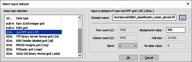
Launch the Fragstats software and import the sieved classification through New > Add layer. Highlight GDAL GeoTIFF grid (.tif) as Data type selection and browse to OBIA_classification_raster_sieved.tif in the dataset selection section as shown in Figure 3. Click on OK.
5. Selection of metrics
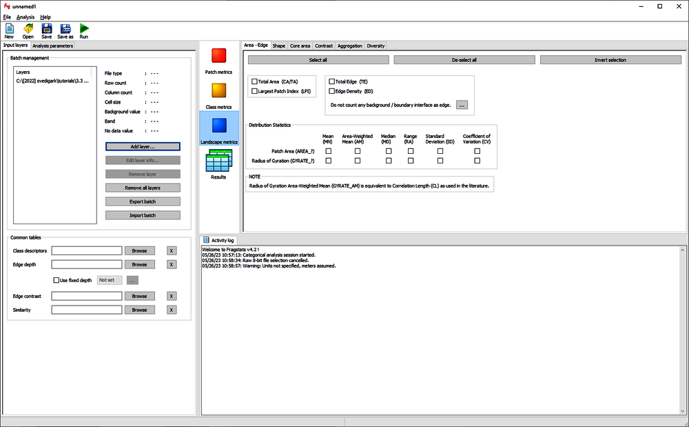
For this tutorial, we are interested in describing the landscape as a whole and the four Land-Use/Land Cover (LULC) classes water, built-up, forest and agriculture/open land in more detail. Click on the blue square to select Landscape metrics first (Figure 4).
Select the following five metrics at landscape level:
• Under the Area-Edge tab, select Largest Patch Index (LPI) and Edge Density (ED)
• Under the Aggregation tab, select Landscape Shape Index (LSI) and Patch Cohesion Index (COHESION)
• Under the Diversity tab, select Simpson’s Diversity Index (SIDI)
As we analyse four different LULC, we are also interested in some metrics that describe each class. Choose Class metrics (the yellow square) and check the following four metrics:
• Under the Area-Edge tab, select Percentage of Landscape (PLAND) and Patch Area (AREA_MN)
• Under the Aggregation tab, select Number of Patches (NP) and Patch Density (PD)
6. Run the model to generate metrics
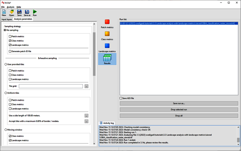
Before the model can be run, we need to specify on what level the analysis shall be performed. Based on the selection of the metrics, we will run the analysis at the landscape and class levels. Check the Class metrics and Landscape metrics boxes under Sampling strategy > No Sampling under the Analysis parameters as shown in Figure 5.
7. Interpreting the results
The results from the calculation are shown below (unnecessary blank spaces removed). At landscape level:
LID, LPI, ED, LSI, COHESION, SIDI
C:\temp\classification.tif, 28.0150, 59.3789, 95.3228, 99.8559, 0.6490
At class level:
LID, TYPE, PLAND, NP, PD, AREA_MN
C:\temp\classification.tif, cls_3, 44.5696, 4056.0000, 1.0048, 44.3549
C:\temp\classification.tif, cls_4, 16.8870, 11758.0000, 2.9129, 5.7972
C:\temp\classification.tif, cls_2, 3.5252, 15332.0000, 3.7984, 0.9281
C:\temp\classification.tif, cls_1, 35.0182, 820.0000, 0.2031,172.3777
To interpret the results correctly, we need to consult the Fragstats help that we downloaded before (McGarigal 2015) for range and of possible values for each metric and explanation thereof.
At the landscape level, a LPI of 28.015 means, that 28.015% of the landscape are occupied by one single connected patch, in our case the large water body in the south-west (part of lake Vänern). An ED of 59.3789 corresponds to the sum of the lengths (m) of all edge segments in the landscape, divided by the total landscape area (m2), multiplied by 10,000 (to convert to hectares). Note that ED has the same utility and limitations as Total Edge, except that edge density reports edge length on a per unit area basis that facilitates comparison among landscapes of varying size. Whether the information that there are 59 m of edge/ha in itself is useful is up to the user. However, in relation to previous conditions in the same landscape or in relation to other study areas, the value becomes indicative. The LSI provides a standardized measure of total edge or edge density that adjusts for the size of the landscape, or in other words it is an index that expresses the perimeter-to-area ratio for the landscape as a whole and can be considered a measure of landscape complexity. Again, an appraisal of LSI is more meaningful in relation to other data but a value of 95.3228 is indicative for a relatively complex landscape. COHESION equals 1 minus the sum of patch perimeter (in terms of number of cells) divided by the sum of patch perimeter times the square root of patch area (in terms of number of cells) for all patches in the landscape, divided by 1 minus 1 over the square root of the total number of cells in the landscape, multiplied by 100 to convert to a percentage. This is difficult to interpret but assume that the higher the COHESION value, the higher the connectedness within the landscape. SIDI equals 1 minus the sum, across all patch types, of the proportional abundance of each patch type squared. The range is from 0 to 1. A value of 0.6490 indicates a moderately diverse landscape.
At class level, let us first doublecheck what cls_1 to cls_4 as output from Fragstats corresponds to in terms of our classes. We can check that by going back to the class descriptions and colour scheme in QGIS: Cls_1 = Water; Cls_2 = Built-up; Cls_3 = Forest; Cls_4 = Agriculture/open land. We can observe through the PLAND metric, that the dominant class in the landscape is forest, occupying 44.57% of the landscape, followed by water (35.02%), agriculture/open land (16.89%) and built-up areas (3.53%). Water is significantly less fragmented (which makes sense) with only 820 patches (lake Vänern, lakes and streams) in comparison to other classes. Especially built-up space and open land show high numbers of patches. This can be explained through settlements and singular buildings that are not considered connected to each other, at least not at the spatial resolution of 10 m, being too coarse to identify minor roads. Patches of open land/pasture and agricultural fields are not naturally connected as they were converted from forest through human settlers in the past. PD in our case study is somewhat redundant in relation to NP as it relates the number of patches to its respective class area (NP/100 hectares) but can be complementing in different settings. The mean patch area AREA_MN gives an indication of the average size of a patch in a respective class in hectares. Built-up areas are on average about one hectare, corresponding to 10x10 pixels in our image.
How to
As studies in landscape archaeology can cover a broad range of topics, it is not possible to recommend a generic set of LM as the importance of different landscape aspects as indicators varies with the scope of the study. The LM showcased here are commonly applied and are described in detail in the Fragstats Help by McGarigal (2015). The descriptions provided here are taken and shortened from the abovementioned document.
• The Largest Patch Index (LPI) quantifies the percentage of total landscape area comprised by the largest patch. As such, it is a simple measure of dominance.
• Total Edge (TE) is an absolute measure of total edge length of a particular patch type (class level) or of all patch types (landscape level). In applications that involve comparing landscapes of varying size, this index may not be useful. Edge density (ED) standardizes edge to a per unit area basis that facilitates comparisons among landscapes of varying size. However, when comparing landscapes of identical size, total edge and edge density are completely redundant.
• One popular index that subsumes both dispersion and interspersion is Contagion (CONTAG) based on the probability of finding a cell of type i next to a cell of type j. The contagion index is appealing because of the straightforward and intuitive interpretation of this probability.
• The Landscape Shape Index (LSI) index measures the perimeter-to-area ratio for the landscape as a whole. It can be interpreted as a measure of the overall geometric complexity of the landscape. However, it can also be interpreted as a measure of landscape disaggregation – the greater the value of LSI, the more dispersed are the patch types.
• COHESION quantifies the connectivity of habitat as perceived by organisms dispersing in binary landscapes.
• Simpson’s diversity index (SIDI) is a popular measure of diversity in community ecology. SIDI is less sensitive to the presence of rare types and has an interpretation that is much more intuitive than Shannon's index. Specifically, the value of SIDI represents the probability that any two pixels selected at random would be different patch types.
• Percentage of Landscape (PLAND) describes a landscape class’s areal share of the total landscape.
• Number of patches (NP) of a particular patch type is a simple measure of the extent of subdivision or fragmentation of the patch type. Although NP in a class may be fundamentally important to a number of ecological processes, often it has limited interpretive value by itself because it conveys no information about area, distribution, or density of patches. Interpreting NP together with PLAND is a powerful indicator of fragmentation between two datasets from different times. If, e.g., the PLAND value does not change and NP increases, the class has become more fragmented. On the other hand, if NP remains constant but PLAND changes, one can assume that existing patches either shrank or grew in size. Decreasing NP with stable or increasing PLAND indicates an increased connectedness and/or consolidation of a class.
• Patch Density (PD) is a limited, but fundamental, aspect of landscape pattern. PD has the same basic utility as number of patches as an index, except that it expresses number of patches on a per unit area basis that facilitates comparisons among landscapes of varying size.
Reference
Landscape Metrics
LM are tools used in landscape ecology to quantify the spatial characteristics of landscapes. These metrics help in understanding the structure, function, and changes in a landscape over time. They are essential for assessing biodiversity, habitat fragmentation, and the impacts of human activities like urbanization or agriculture. By analyzing aspects like patch size, edge length, or connectivity, LM provide valuable insights for conservation planning, environmental management, and policy-making. They support the identification of critical areas for protection and the evaluation of landscape changes, thereby facilitating sustainable land-use practices and contributing to ecological research.
QGIS
QGIS (formerly known as Quantum GIS) is a free, open-source Geographic Information System (GIS) software that enables users to visualize, analyse, edit, and manage geospatial data on various platforms, including Windows, macOS, Linux, and Android. QGIS supports various vector, raster, and database formats and provides a wide range of geoprocessing tools, cartographic capabilities, and spatial analysis functions. QGIS is developed by the QGIS.org project, which is supported by a large community of contributors, including developers, GIS professionals, and users. The project aims to provide an accessible and user-friendly GIS platform for both beginners and advanced users. QGIS is a powerful GIS platform suitable for various applications, such as environmental management, urban planning, disaster response, and natural resource management. Its open-source nature and active community make it an attractive alternative to proprietary GIS software.
Sieve
According to the QGIS documentation, the Sieve function “removes raster polygons smaller than a provided threshold size (in pixels) and replaces them with the pixel value of the largest neighbour polygon.” It is useful if one has a large amount of small areas on a raster map that need to be removed.
Fragstats
Fragstats is a program developed to quantify landscape structure. It offers a comprehensive choice of LM and was designed to be as versatile as possible. The program is almost completely automated and thus requires little technical training (McGarigal and Marks 1995). Further information is given in McGarigal et al. (2012).
Explanation
LM are quantitative measures used to describe the composition, structure, and configuration of landscapes. These metrics help landscape ecologists, planners, and landscape archaeologists to understand and analyse the spatial patterns within landscapes and evaluate the potential impacts of natural and human-induced changes. They are essential for understanding landscape patterns and processes, informing landscape management and conservation strategies, and guiding landscape planning and design. They are typically calculated using GIS tools and software, along with spatial data on land cover, land use, or other relevant landscape features. For the foundations of LM, the works of Urban et al. (1987) and their more recent applications Uuemaa (2009) are good starting points.
LM can be broadly categorized into three groups:
1. Composition metrics: These metrics describe the overall makeup of a landscape, focusing on the presence and abundance of different elements or features, such as land cover types, ecosystems, or cultural features. Examples of composition metrics include the proportion of each land cover type, the total area of specific land cover classes, and the diversity of land cover types present.
2. Configuration metrics: Configuration metrics describe the spatial arrangement of landscape elements, including the shape, size, and distribution of patches or features within the landscape. Examples of configuration metrics include patch density (number of patches per unit area), edge density (length of patch edges per unit area), and contiguity (the degree to which patches of the same type are connected).
3. Connectivity metrics: Connectivity metrics quantify the degree to which landscape elements are connected or linked, either through physical adjacency or functional relationships (such as wildlife corridors or hydrological networks). Examples of connectivity metrics include connectivity index (measures the functional connectivity based on the distance between patches), and nearest neighbour distance (average distance to the nearest neighbouring patch of the same type).
The theoretical and conceptual basis for understanding landscape structure, function and change originated from the field of landscape ecology (Forman & Godron 1986). Habitat fragmentation is a threat to species and in order to conserve and maintain these habitats, management of entire landscapes and not just of several components is needed. LM are a well-known concept that can be summarized as a range of variables that describe particular aspects of landscape patterns, interactions among patches within a landscape mosaic, and the change of patterns and interactions over time. One issue related to applying the concept of LM is the effect of changing landscape scale on the metrics. An attempt to investigate the relationships between pattern indices and changing landscape scale has been undertaken by Wu et al. (2002), where the responses of several commonly used LM to changing grain size, extent, and the direction of analysis was investigated.
As mentioned in the previous section, the selection of metrics is context-dependent and there is no universal set of metrics that always should be used. In many studies, around five metrics are used to describe the landscape and its changes as a whole, often including both composition and configuration metrics. Using LM for archaeological purposes is an innovative approach and the following suggestions can give the user a hint on when to use which metrics:
• Patch Density (PD): This metric calculates the number of patches per unit area. In archaeology, it can be used to understand the distribution density of archaeological sites or features within a given area.
• Largest Patch Index (LPI): This measures the percentage of the landscape comprised by the largest patch. For archaeological purposes, LPI can help in identifying dominant site types or cultural features within a landscape, indicating areas of major historical activity.
• Edge Density (ED): ED measures the length of the edge of patches per unit area. In archaeology, this can be useful for understanding the interaction between different land uses or cultural areas, such as the boundary between agricultural and residential areas in ancient settlements.
• Shannon's Diversity Index (SHDI) and Simpson's Diversity Index (SIDI): These indices measure landscape diversity. They could be applied in archaeology to assess the diversity of site types or cultural features within a landscape, which might indicate a varied use of the land or the presence of different cultural groups.
• Mean Patch Size (MPS): This metric calculates the average size of patches. In an archaeological context, it might be used to understand the average size of habitation sites or cultural features, providing insight into settlement patterns.
• Contagion Index (CONTAG): This measures the degree to which patch types are aggregated or clumped. Archaeologically, this could be insightful for examining the degree of clustering of sites, which might reflect social or environmental factors.
• Landscape Shape Index (LSI): LSI assesses the complexity of shape for patches. In archaeology, more complex shapes might indicate prolonged human modification of the landscape.
• Core Area Metrics: These metrics focus on the area of patches excluding the edge. They can be used in archaeology to focus on the central, most used parts of a site, potentially identifying core areas of activity.
As stated above, each of these metrics can provide different insights into the archaeological landscape, depending on a specific research question. It's crucial to select metrics that align with your objectives, whether you're studying settlement patterns, land use, cultural interactions, or other aspects of the archaeological record.
There are limited studies on the use of LM in archaeology although they have a huge potential in describing past and present composition and configuration of landscapes alongside their changes. The value in using LM for describing anthropological and historical data was highlighted in Foster II et al. (2016). Recently, Zheng et al. (2020) employed several metrics in a landscape visibility and viewshed fragmentation analysis in an ancient metropolitan area.
In summary, the benefit of using LM in archaeological applications lies in their ability to quantify and compare the spatial relations of land use classes, human artifacts and settlements to their surroundings.
References
Forman, R. T. T., & Godron, M. (1986). Landscape Ecology. John Wiley and Sons, New York.
Foster II, H. T., Goldstein, D. J., & Paciulli, L. M. (2016). How Archaeology and the Historical Sciences Can Save the World. VIEWING THE FUTURE IN THE PAST, 1.
Mcgarigal, K. (2015). FRAGSTATS Help. www.umass.edu/landeco/research/fragstats/documents/fragstats.help.4.2.pdf. McGarigal, K., Cushman, S. A., & Ene, E. (2012). FRAGSTATS v4: Spatial pattern analysis program for categorical and continuous maps (Computer software program produced by the authors at the University of Massachusetts, Amherst). Retrieved from: www.umass.edu landeco/research/fragstats/fragstats.html
McGarigal, K. and Marks, B. (1995). FRAGSTATS: spatial pattern analysis program for quantifying landscape structure (Vol. 351). US Department of Agriculture, Forest Service, Pacific Northwest Research Station.
Urban, D. L., O’Neill, R. V., Shugart Jr., H. H. (1987): Landscape ecology: a hierarchical perspective can help scientists understand spatial patterns. BioScience, 37, 119-127.
Uuemaa, E., Antrop, M., Roosaare, J., Marja, R., & Mander, Ü. (2009). Landscape metrics and indices: An overview of their use in landscape research. Living Reviews in Landscape Research, 3(1), 1-28.
Wu, J., Shen, W., Sun, W., & Tueller, P. T. (2002). Empirical patterns of the effects of changing scale on landscape metrics. Landscape ecology, 17, 761-782.
Zheng, M., Tang, W., Ogundiran, A., Chen, T., & Yang, J. (2020). Parallel landscape visibility analysis: A case study in archaeology. High Performance Computing for Geospatial Applications, 77-96.