Satellite image processing
Image processing of Sentinel-1 SAR (S-1) and Sentinel-2 multispectral (MSI) (S-2) data for applications in landscape archaeology
Author: Jan Haas - Last update 2023-08-31
Citation:
Haas, J. (2024). Image processing of Sentinel-1 SAR (S-1) and Sentinel-2 multispectral (MSI) (S-2) data for applications in landscape archaeology. Zenodo. doi.org/10.5281/zenodo.10687538
Introduction
This tutorial is aimed at providing the user with knowledge and practical skills on satellite image acquisition, pre-processing and export for purposes within landscape archaeology. The methodological steps might vary depending on the satellite sensor. The processing steps described in this tutorial are developed and showcased for two satellite types that are actively run by the European Space Agency (ESA), i.e., Sentinel-1 (SAR) and Sentinel-2 (MSI). The tutorial makes use of ESA’s Sentinels Application Platform SNAP toolbox. All data and software are free of charge. After completing this tutorial, the user should be able to find, download and pre-process spaceborne SAR and multispectral data from two popular Earth Observation satellites. The user should have gained some basic understanding of the steps needed to prepare satellite data for analysis, have attained some familiarity with SNAP and should be able to produce a GeoTIFF image that can further be used for landscape archaeological applications, e.g., visual image interpretation, image classification, derivation of a variety of indices or change detection.
Tutorial
This tutorial will guide you through the process of downloading S-1 and S-2 data from the Copernicus Open Access Hub, installing the SNAP software, processing SAR and multispectral data and exporting them in GeoTiff-format.
1. Data download from the Copernicus Open Access Hub
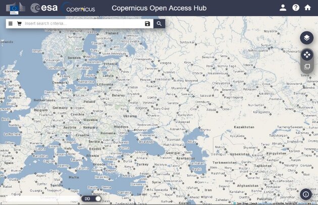
1.1 Visit the Copernicus Open Access Hub website (Figure 1)
1.2 Register for an account if you have not done so already.
1.3 Log in and specify your region of interest with the tool to the right-hand side (Figure 2) through drawing a polygon. Alternatively, you can upload a shapefile delineating your region of interest.

1.4 Search for data, by specifying the desired parameters according to the parameters in Figure 3.
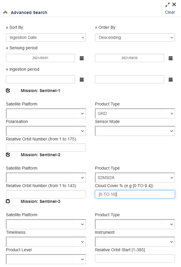
Search for S-1 data using the parameters Sensing period and Product Type. Specify Sensing period and chose Product Type as GRD (Ground Range Detected).
Regarding the acquisition of S-2 data, specify Sensing period and set Product Type as S2MSI2A. Adjust Sensing period and set Cloud Cover % to [0 TO 10] percent. Adjust if no appropriate images can be found.
Figure 4 shows the result of a search with parameters specified in Figure 3.
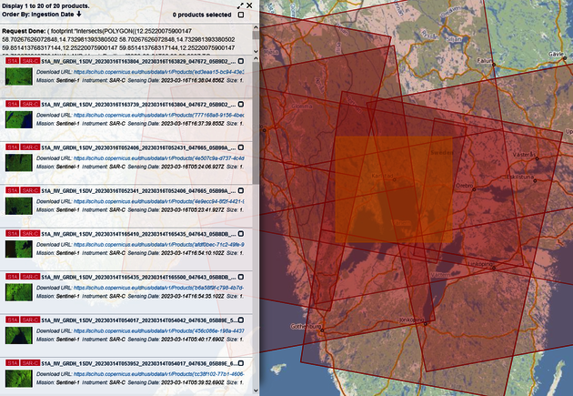
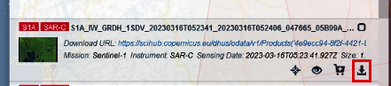
1.5 From the images that are found, select the one over the region of interest and download follow the download link in the lower right corner to obtain the file (Figure 5).
2. Software download and installation of the SNAP
2.1 Visit the ESA Sentinel-2 SNAP toolbox website. Select the Sentinel Toolboxes and download the appropriate version for your operating system.
2.2 Follow the installation instructions provided in the installation wizard.
3. S-1 data processing
3.1 Import data
Launch SNAP and Click on File > Import > SAR Sensors > SENTINEL-1 and browse to your downloaded .zip file to import the data.
3.2 Apply orbit file
Go to the Radar tab and click on Apply orbit file. Leave the Processing parameters untouched. Choose the radar image as source file and save the orbit file in the same directory. Keep the automatically generated file name …_Orb. Save in the BEAM-DIMAP format. Click on Run to generate the file.
3.3 GRD border noise removal (optional)
Go to the Radar tab and click on Sentinel-1 TOPS and choose S-1 Remove GRD Border Noise. Leave the processing parameters untouched. Choose the latest radar image as source file and save the orbit file in the same directory. Keep the automatically generated file name … _Orb_Bdr. Save in the BEAM-DIMAP format. Click on Run to generate the file.
3.4 Thermal noise removal
Go to the Radar tab and click on Radiometric and choose S-1 Thermal Noise Removal. Leave the processing parameters untouched. Choose the latest radar image as source file and save the orbit file in the same directory. Keep the automatically generated file name … _Orb_Bdr_tnr. Save in the BEAM-DIMAP format. Click on Run to generate the file.
3.5 Speckle filtering
Go to the Radar tab and click on Radiometric and choose Speckle filtering > Single Product Speckle Filter. If you have more image acquisitions you can choose Multi-spectral Spectral Filter. Go to the processing parameters and chose a speckle filter. Choose the latest radar image as source file and save the speckle filtered file in the same directory. Keep the automatically generated file name, e.g. …_Orb_Bdr_tnr_SpkLee. Save in the BEAM-DIMAP format. Click on Run to generate the file.
3.6 Radiometric calibration
Go to the Radar tab and click on Radiometric and choose Calibrate. Leave the processing parameters untouched. Choose the latest radar image as source file and save the file in the same directory. Keep the automatically generated file name …Orb_Bdr_tnr_SpkLee_Cal. Save in the BEAM-DIMAP format. Click on Run to generate the file.
3.7 Terrain correction
Go to the Radar tab and click on Geometric and choose Terrain Correction > Range Doppler Terrain Correction. Specify the Digital Elevation Model (DEM) and leave the other processing parameters untouched. Choose the one with the highest spatial resolution available, e.g., Copernicus 30m Global DEM (Auto Download). In the Map Projection Settings choose Custom CRS with the UTM / WGS84(Automatic) Projection. Choose the latest radar image as source file and save the file in the same directory. Keep the automatically generated file name …Orb_Bdr_tnr_SpkLee_Cal_TC. Save in the BEAM-DIMAP format. Click on Run to generate the file.
3.8 Stack (optional if you want to combine one or more images)
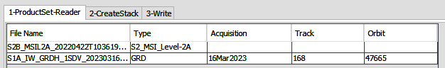
Go to Radar > Coregistration > Stack Tools > Create Stack. In the 1-ProductSet-Reader, add two or more images. If you use a S-2 image, put it above the S-1 image (Figure 6).
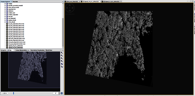
In the 2-CreateStack dialogue, choose NEAREST_NEIGHBOUR as Resampling Type, Orbit as Initial Offset Method and specify the Output extent as Minimum. In the 3-Write section, give the output file an appropriate name, e.g. S1-S2_stack and save it in the BEAM-DIMAP-format. Click on Run. The output of the stack operation is displayed in Figure 7. Note that an irregular data frame has been created covering just overlapping areas and that all information from two sensors is retained in the Product Explorer window.
3.9 Subset (optional)
Go to Raster > Subset. In the Spatial Subset tab, modify the blue rectangle to the left according to define the bounding box of your area of interest. Select the image bands that you need for your particular application, e.g., B1-B12 from S-2 and the two Sigma0 bands from S-1. Select no derived products from the Tie-Point Grid subset unless you need them for a particular purpose. Click on OK. A new product has appeared in the Product Explorer.
3.10 Export to GeoTIFF format
Right click on the latest file in the Product Explorer and then on Save as…. Save in the BEAM-DIMAP format first, e.g., as subset_0_of_S1-S2_stack.dim. As a last step, go to File > Export > GeoTIFF / BigTIFF and specify the output file name and location. Click on OK to start the export process.
4. S-2 pre-processing
4.1 Data import
Launch SNAP and go to File > Import > Optical Sensors > Sentinel-2 > S2-MSI L2A and browse to the Sentinel-2 folder you downloaded earlier. Open the file called MTD_MSIL2A.xml. Double-click B1-B12 in the Product Explorer to visualize the data.
4.2 Resampling
Go to Raster > Geometric Operations and open the Resample operation to increase the spatial resolution of image bands. Under the Resampling Parameters tab, choose B2 as input to By reference band from source. An overview of all Sentinel-2 bands and resolutions is provided in the Reference section. Keep all other parameters and name the output file as suggested (_resampled) and click on Run.
4.3 Stack
(optional if you want to combine one or more images) See section 3.8
4.4 Subset
(optional) See section 3.9
4.5 Export to GeoTIFF format
See section 3.10
How to
This section covers some topics that need consideration from the analyst when selecting data and choosing parameters. A lot of information that is presented here can also be found in the help section for the respective module in SNAP.
S-1 data and processing
Image download
When selecting download parameters, one needs to decide what sensor mode and polarizations are best suited for the task at hand. The choice of polarizations and sensor modes will depend on the specific research objectives and features of the landscape being studied. Some of the commonly used SAR polarizations and sensor modes are:
1. HH (Horizontal-Horizontal) polarization: This polarization is commonly used for vegetation mapping and monitoring, as well as for identifying soil moisture and surface roughness.
2. VV (Vertical-Vertical) polarization: This polarization is commonly used for mapping land cover and identifying changes in surface roughness.
3. HV (Horizontal-Vertical) polarization: This polarization is commonly used for detecting and mapping soil moisture and changes in vegetation cover.
4. VH (Vertical-Horizontal) polarization: This polarization is less commonly used in landscape archaeology, but can be useful for identifying changes in vegetation cover.
In terms of sensor modes, the most commonly used mode in landscape archaeology is the Interferometric Wide Swath (IW) mode, which provides high-resolution images and is well-suited for mapping and monitoring of land cover and surface features. Other modes such as Stripmap (SM) and Extra-Wide Swath (EW) modes may also be used in certain applications, depending on the spatial resolution and coverage area required.
Apply orbit file
The orbit state vectors provided in the metadata of a SAR product are generally not accurate and can be refined with the precise orbit files which are available days-to-weeks after the generation of the product.
The orbit file provides accurate satellite position and velocity information. Based on this information, the orbit state vectors in the abstract metadata of the product are updated. The operator currently only supports ASAR, ERS and Sentinel-1 products. To refine the orbit state vectors, the following steps are performed:
1. Get the start time of the source product;
2. Find orbit file with user specified type and the product start time;
3. For each orbit state vector in the metadata, get its UTM time;
4. Compute new orbit state vector for the UTM time using interpolation.
GRD border noise removal (optional)
Use this step if you are interested in the whole scene or if you intend to mosaic the image together with adjacent Sentinel-1 tiles.
The Sentinel-1 (S-1) Instrument Processing Facility (IPF) is responsible for generating the complete family of Level-1 and Level-2 operation products. The processing of the RAW data into L1 products features number of processing steps leading to artefacts at the image borders.
These processing steps are mainly the azimuth and /range compression and the sampling start time changes handling that is necessary to compensate for the change of earth curvature. The latter is generating a number of leading and trailing “no-value” samples that depends on the data-take length that can be of several minutes. The former creates radiometric artefacts complicating the detection of the “no-value” samples. These “no-value” pixels are not null but contain very low values which complicates the masking based on thresholding.
Thermal noise removal
Thermal noise correction can be applied to Sentinel-1 Level-1 SLC products as well as Level-1 GRD products which have not already been corrected. The operator can also remove this correction based on the product annotations (i.e. to re-introduce the noise signal that was removed). Product annotations will be updated accordingly to allow for re-application of the correction. Level-1 products provide a noise LUT for each measurement data set. The values in the de-noise LUT, provided in linear power, can be used to derive calibrated noise profiles matching the calibrated GRD data. Bi-linear interpolation is used for any pixels that fall between points in the LUT.
Speckle filtering
SAR images have inherent salt and pepper like texturing called speckles which degrade the quality of the image and make interpretation of features more difficult. Speckles are caused by random constructive and destructive interference of the de-phased but coherent return waves scattered by the elementary scatters within each resolution cell. Speckle noise reduction can be applied either by spatial filtering or multilook processing. For respective speckle filters and their parametrization, check the SNAP help section. Test different speckle filters and review the results. Depending on your imagery and application domain, appropriate filters need to be chosen. Visually inspect the results from the different speckle filtering operations and chose the best one.
When choosing a speckle filter, there are several options to consider. The choice of speckle filter will depend on the specific features of the SAR data being processed and the research objectives. Here are a few options to consider:
1. Lee Filter: The Lee filter is a popular choice for SAR data processing in landscape archaeology. It is a simple filter that works well in areas with homogeneous backscatter, such as agricultural fields, and can preserve spatial details while reducing speckle noise.
2. Gamma MAP Filter: The Gamma Maximum a Posteriori (MAP) filter is another commonly used speckle filter for SAR data processing. It is a Bayesian filter that uses a statistical model to estimate the original backscatter intensity from the speckled image. It works well for areas with complex features, such as urban areas or forests.
3. Frost Filter: The Frost filter is a nonlinear filter that can suppress speckle noise while preserving image details. It works well in areas with varying backscatter, such as coastal zones or mountainous areas.
4. Median Filter: The Median filter is a simple filter that can effectively reduce speckle noise in SAR images while preserving edges and textures. It is a good choice for areas with a high degree of speckle noise, such as areas with strong backscatter variations.
In summary, when choosing a speckle filter for landscape archaeology, the choice will depend on the specific features of the SAR data and research objectives of the archaeologist. The Lee, Gamma MAP, Frost, and Median filters are some commonly used filters that may be appropriate for different types of SAR data.
Radiometric calibration
This step corrects for variations in the signal intensity caused by the radar system, atmospheric conditions, and other factors. The objective of SAR calibration is to provide imagery in which the pixel values can be directly related to the radar backscatter of the scene. Though uncalibrated SAR imagery is sufficient for qualitative use, calibrated SAR images are essential to quantitative use of SAR data.
Typical SAR data processing, which produces level 1 images, does not include radiometric corrections and significant radiometric bias remains. Therefore, it is necessary to apply the radiometric correction to SAR images so that the pixel values of the SAR images truly represent the radar backscatter of the reflecting surface. The radiometric correction is also necessary for the comparison of SAR images acquired with different sensors, or acquired from the same sensor but at different times, in different modes, or processed by different processors.
The Calibrate operator performs different calibrations deriving the sigma nought images. The Sigma naught (Sigma0) image channels are the ones that should be used for image classification, e.g. Sigma0_VH and Sigma_VV that can be found in the file when you open the Bands folder of the image in SNAP. Optionally gamma nought and beta nought images can also be created.
Terrain correction
This step corrects for distortions in the SAR image caused by the terrain relief and the sensor's viewing geometry, which can affect the interpretation of the archaeological features. Due to topographical variations of a scene and the tilt of the satellite sensor, distances can be distorted in the SAR images. Image data not directly at the sensor’s Nadir location will have some distortion, effects that are also known as forshortening and layover. Terrain corrections are intended to compensate for these distortions so that the geometric representation of the image will be as close as possible to the real world. Terrain Correction is a necessary step in image analysis and it allows geometric overlays of data from different sensors and/or geometries. Especially in mountainous areas, where large differences in relief energy exist, terrain correction is needed.
Create Stack (optional)
Use this function if you have multiple images over the same area that you want to analyse at the same time. It is, from an image classification point of view considered beneficial to use multi-sensor data to derive landcover and land use (LULC) information, e.g., one could use both Sentinel-1 and Sentinel-2 data at the same time. Create Stack is a component of coregistration. The Create Stack Operator allows collocating two spatially overlapping products. Collocating two products implies that the pixel values of one product (the secondary) are resampled into the geographical raster of the other (the reference).
When two products are collocated, the band data of the secondary product is resampled into the geographical raster of the reference product. In order to establish a mapping between the samples in the reference and the secondary rasters, the geographical position of a reference sample is used to find the corresponding sample in the secondary raster. If there is no sample for a requested geographical position, the reference sample is set to the no-data value which was defined for the secondary band. The collocation algorithm requires accurate geopositioning information for both reference and secondary products. When necessary, accurate geopositioning information may be provided by ground control points. The metadata for the stack product is copied from the metadata of the reference product. For further information on Create Stack and Resampling Options, consult the Help Section in SNAP. Creating the stack used in this tutorial takes some time (19.7 minutes on a Intel(R) Core(TM) i9-10885H CPU @ 2.40GHz; 2.40 GHz mobile workstation with 128 GB RAM and a NVIDIA Quadro RTX 5000 GPU). By choosing Minimum as Output extent, only the overlapping areas will be mapped into a new file, thus drastically reducing processing times.
Subset (optimal)
Creating subsets of your data, whether stacked or not, can dramatically decrease image size and thus processing times. It can get rid of NoData areas around image boundaries and but just focusing on a particular area of interest, remove LULC data that is not relevant to the study, thus simplifying the classification task at hand.
S-2 data processing
As we acquired the Level-2A product, not all pre-processing steps are required. Level-2A processing includes a Scene Classification and an Atmospheric Correction applied to Top-Of-Atmosphere (TOA) Level-1C orthoimage products. Level-2A main output is an orthoimage atmospherically corrected, Surface Reflectance product. Information on Sentinel-2 pre-processing levels can be found here.
Geometric distortions
Geometric distortions in multispectral satellite data refer to any changes in the spatial position or shape of features on the ground that are introduced during the image acquisition process. These distortions can occur due to a variety of factors, such as variations in satellite altitude, rotation, and sensor misalignment. Geometric distortions can have a significant impact on the accuracy of image interpretation and analysis, particularly for applications that require precise spatial information, such as land cover mapping, change detection, and environmental monitoring.
To correct geometric distortions in multispectral satellite data, several methods can be used. These include:
Orthorectification: This involves the use of ground control points (GCPs) to adjust the position of the image pixels to their correct geographic coordinates. Orthorectification requires accurate information on the topography and terrain of the image area, and typically involves the use of digital elevation models (DEMs) to correct for variations in terrain elevation.
Resampling: Resampling is a process that involves changing the spacing and position of the pixels in the image to match a predefined grid or coordinate system. Resampling is often used to correct distortions caused by sensor misalignment or changes in the satellite altitude.
Image registration: Image registration involves the alignment of two or more images to the same coordinate system. This can be done by identifying common features in the images, such as road intersections or building corners, and using these to align the images.
Sensor modeling: Sensor modeling involves the use of mathematical models to correct for distortions caused by sensor characteristics, such as lens distortion or sensor misalignment.
Overall, correcting geometric distortions in multispectral satellite data is an important step in ensuring the accuracy and reliability of image analysis and interpretation, particularly for applications that require precise spatial information. The choice of correction method will depend on the specific data and research objectives, as well as the accuracy required for the particular application.
Spectral distortions
Spectral distortions in multispectral satellite data refer to changes in the spectral response of an image caused by variations in atmospheric conditions, sensor calibration, and other factors. These distortions can lead to inaccurate or inconsistent measurements of the reflected or emitted radiation from the Earth's surface, which can affect the accuracy of image interpretation and analysis.
To correct for spectral distortions in multispectral satellite data, several methods can be used. These include:
Atmospheric correction: Atmospheric correction involves the removal of atmospheric effects on the image data. This is done by estimating the amount of atmospheric scattering and absorption, and subtracting this from the image data. Several algorithms are available for atmospheric correction, including FLAASH, ATCOR, and MODTRAN.
Radiometric calibration: Radiometric calibration involves the adjustment of image data to correct for variations in sensor response, such as changes in sensor gain or bias. This is typically done using calibration targets or ground measurements to establish a relationship between the measured signal and the true radiance or reflectance.
Spectral calibration: Spectral calibration involves the adjustment of the spectral response of the image data to match a known spectral reference. This is typically done using spectral calibration targets, such as lamps or filters, to establish a relationship between the measured spectral response and the true spectral response.
Cross-sensor normalization: Cross-sensor normalization involves the adjustment of image data from different sensors to match a common spectral reference. This is done by establishing a relationship between the spectral response of the different sensors, and applying a correction factor to align the spectral response (see also relative atmospheric correction).
Overall, correcting spectral distortions in multispectral satellite data is an important step in ensuring the accuracy and reliability of image analysis and interpretation. The choice of correction method will depend on the specific data and research objectives, as well as the accuracy required for the particular application.
Atmospheric effects, absolute and relative
Atmospheric correction is a critical step in the pre-processing of remote sensing data, particularly in optical remote sensing where atmospheric effects can cause significant distortions in the measured signal. The atmospheric correction process aims to remove the effects of atmospheric scattering and absorption on the recorded signal, in order to obtain more accurate and meaningful information about the surface features.
There are two main approaches to atmospheric correction: absolute atmospheric correction and relative atmospheric correction.
Absolute atmospheric correction involves the estimation of atmospheric parameters such as aerosol optical thickness and water vapor content, and their application to correct the recorded signal for atmospheric effects. Absolute atmospheric correction requires accurate knowledge of the atmospheric conditions at the time of the image acquisition, which can be obtained from in situ measurements or atmospheric models. Absolute atmospheric correction is particularly important for quantitative applications, such as vegetation indices or land cover classification, where accurate radiometric calibration is essential.
Relative atmospheric correction, on the other hand, involves the removal of the atmospheric effects by comparing the reflectance values of one image with the ones of another image over the same are. Relative atmospheric correction is less accurate than absolute atmospheric correction, but it is often used when accurate atmospheric measurements are not available or when the focus is on relative changes in the reflectance values, rather than absolute values, e.g. it is essential for change detection of vegetation features.
Both absolute and relative atmospheric correction are needed in order to obtain accurate and meaningful information from remote sensing data. The choice of which method to use will depend on the specific research objectives, available atmospheric data, and the accuracy required for the particular application.
Clouds
Clouds can be a significant problem in multispectral image data as they can obscure the land surface features and interfere with image interpretation and analysis. Here are some common approaches for handling clouds in multispectral image data:
Cloud masking: This involves identifying and masking out the cloud-affected pixels in the image. Several methods can be used to detect clouds, including thresholding, supervised classification, and machine learning techniques. The masked areas can then be filled in or excluded from further analysis.
Cloud removal: This involves removing the clouds from the image data, typically by interpolating the values of the affected pixels based on nearby, cloud-free pixels. Several methods can be used for cloud removal, including linear and nonlinear interpolation, filtering, and spectral unmixing. However, it is important to note that cloud removal can introduce errors and artifacts into the image data and should be used with caution.
Cloud compositing: This involves creating a composite image from multiple cloud-free scenes acquired at different times or dates. This can be done manually or using automated techniques, such as the Maximum Value Composite (MVC) or Minimum Noise Fraction (MNF) methods. The resulting composite image can then be used for analysis and interpretation, with the caveat that the composite may not accurately represent the land surface at any single point in time.
Overall, the approach for handling clouds in multispectral image data will depend on the specific research objectives, the accuracy requirements, and the availability of cloud-free data. It is important to carefully evaluate and document the methods used for cloud handling in order to ensure the quality and reliability of the results.
Shadows
Shadows can also be problematic in multispectral image data, particularly in areas with significant relief or steep topography. Here are some common approaches for handling shadows in multispectral image data:
Shadow masking: This involves identifying and masking out the shadow-affected pixels in the image. Several methods can be used to detect shadows, including thresholding, supervised classification, and machine learning techniques. The masked areas can then be filled in or excluded from further analysis.
Shadow removal: This involves removing the shadows from the image data, typically by interpolating the values of the affected pixels based on nearby, shadow-free pixels. Several methods can be used for shadow removal, including linear and nonlinear interpolation, filtering, and spectral unmixing. However, it is important to note that shadow removal can introduce errors and artifacts into the image data and should be used with caution.
Radiometric normalization: This involves adjusting the radiometric values of the shadow-affected pixels to account for the reduced reflectance caused by the shadow. This can be done using empirical or physically-based models, such as the Li-Strahler geometric-optical model. Radiometric normalization can help to mitigate the effects of shadows on image analysis, but it does not completely remove the shadows.
Overall, the approach for handling shadows in multispectral image data will depend on the specific research objectives, the accuracy requirements, and the availability of shadow-free data. It is important to carefully evaluate and document the methods used for shadow handling in order to ensure the quality and reliability of the results.
The Sentinel-2 MSI instrument
Sentinel-2 data has been used in various applications in landscape archaeology, including mapping and detecting archaeological features, and analyzing landscape patterns. In general, Sentinel-2 bands that are useful for landscape archaeology applications are those that are sensitive to vegetation, soil, and moisture characteristics. Some of the commonly used Sentinel-2 bands for landscape archaeology are:
1. Red (B4): This band is useful for distinguishing vegetation from soil and water, and for identifying changes in vegetation cover.
2. Near-Infrared (B8): This band is sensitive to vegetation health and density and can be used for vegetation mapping and monitoring.
3. Shortwave Infrared (B11 and B12): These bands are useful for mapping and identifying changes in soil moisture, and can also be used for detecting changes in land cover.
4. Green (B3): This band is sensitive to chlorophyll content in vegetation and can be used for vegetation mapping and monitoring.
5. Blue (B2): This band is useful for detecting changes in water bodies, and for mapping and monitoring of water resources.
In addition to these bands, some studies have also used Sentinel-2's spectral indices, such as the Normalized Difference Vegetation Index (NDVI) and the Enhanced Vegetation Index (EVI), which can provide additional information on vegetation health and density. All in all, Sentinel-2 bands that are useful for landscape archaeology include those that are sensitive to vegetation, soil, and moisture characteristics, such as the Red, Near-Infrared, Shortwave Infrared, Green, and Blue bands. The use of spectral indices such as NDVI and EVI can also provide additional information on vegetation health and density.
Knowing the capability and limitation of your underlying data is important for making the right decisions for your analysis. S-2 provides data at 3 spatial resolutions and different wavelengths:
• 10 m: containing spectral bands 2, 3, 4 , 8, a True Colour Image (TCI) and an AOT and WVP maps resampled from 20 m.
• 20 m: containing spectral bands 1 - 7, the bands 8A, 11 and 12, a True Colour Image (TCI), a Scene Classification (SCL) map and an AOT and WVP map. The band B8 is omitted as B8A provides more precise spectral information.
• 60 m: containing all components of the 20 m product resampled to 60 m and additionally the bands 1 and 9, a True Colour Image (TCI), a Scene Classification (SCL) map and an AOT and WVP map. The cirrus band 10 is omitted, as it does not contain surface information.
Reference
Copernicus
Copernicus is the Earth observation component of the European Union’s Space programme, looking at our planet and its environment to benefit all European citizens. It offers information services that draw from satellite Earth Observation and in-situ (non-space) data. The European Commission manages the Programme. It is implemented in partnership with the Member States, the European Space Agency (ESA), the European Organisation for the Exploitation of Meteorological Satellites (EUMETSAT), the European Centre for Medium-Range Weather Forecasts (ECMWF), EU Agencies and Mercator Océan. Vast amounts of global data from satellites and ground-based, airborne, and seaborne measurement systems provide information to help service providers, public authorities, and other international organisations improve European citizens' quality of life and beyond. The information services provided are free and openly accessible to users (https://www.copernicus.eu/en/about-copernicus).
Sentinel-1
Sentinel-1 is a European Space Agency (ESA) Earth observation satellite mission that provides continuous all-weather day-and-night radar imagery. It is a useful tool for landscape archaeology because it can penetrate through vegetation and capture sub-surface features.
Sentinel-2
Sentinel-2 is a European Space Agency (ESA) Earth observation satellite mission that provides multispectral data for a wide range of applications, including landscape archaeology. The Sentinel-2 mission provides high-resolution imagery with 13 spectral bands, making it a powerful tool for remote sensing analysis. Sentinel-2 image pre-processing requires less steps than Sentinel-1 data, as we downloaded the level 2A product where several processing steps have already been performed, such as a scene classification and an atmospheric correction to the top-of-atmosphere (TOA) level-1C orthoimage product. The level-2A main output is an atmospherically corrected orthoimage surface reflectance product.
SNAP
SNAP is an open source common architecture for ESA Toolboxes ideal for the exploitation of Earth Observation data, jointly developed by Brockmann Consult, SkyWatch and C-S. The SNAP architecture is ideal for Earth Observation processing and analysis.
Explanation
The use of Sentineal-1 SAR and Sentinel-2 MSI data for landscape archaeology
The use of SAR data in landscape archaeology has several advantages over other remote sensing techniques. SAR data can penetrate through vegetation, soil, and even water, which makes it useful for detecting buried archaeological remains and features that are not visible in optical or infrared images. SAR data can also reveal differences in soil moisture and surface roughness, which can help identify buried features, such as ditches, walls, and even ancient roads. SAR data is especially useful in areas with dense vegetation, such as forests and jungles, where traditional remote sensing methods may fail to detect archaeological features due to the high level of vegetation cover. SAR can also be used to identify and map land cover changes, which can be important for understanding the impact of human activity on the landscape over time. Recent studies that use Sentinel-1 SAR in particular have shown the potential of SAR to detect and map archaeological features can be found in e.g., Michenot et al. (2021), Agapiou (2020), Tapete & Cigna (2017) and Elfadaly et al. (2020). Overall, SAR data has proven to be a valuable tool for archaeologists in landscape archaeology, providing a new perspective on the hidden features and structures that lie beneath the earth's surface. Comprehensive overviews of SAR for landscape archaeology can be found in Chen et al. (2017) and Tapete & Cigna (2017).
Multispectral remote sensing is a powerful tool for landscape archaeology, as it can provide valuable information on the composition and characteristics of the landscape over time. Multispectral sensors capture light in different bands across the electromagnetic spectrum, from visible light to near-infrared and thermal radiation. By analyzing the reflectance or emissivity patterns of different materials in the landscape, multispectral remote sensing can help identify and map archaeological features, such as settlements, fortifications, agricultural fields, and burial sites, even in areas with dense vegetation or challenging environmental conditions. Multispectral remote sensing can also provide important information on the environmental and climatic factors that influenced human settlement and land use patterns in the past. For example, by analyzing the reflectance patterns of vegetation, multispectral remote sensing can help reconstruct past land cover and land use changes, such as deforestation, land clearance, and agricultural expansion. Similarly, by analyzing the thermal patterns of the landscape, multispectral remote sensing can help reconstruct past climate conditions and their impact on human settlement and agricultural productivity. Overall, multispectral remote sensing has the potential to revolutionize landscape archaeology, by providing a new perspective on the hidden structures and features that lie beneath the earth's surface, and by enabling a more holistic and interdisciplinary approach to understanding the human-environment interactions that shaped the landscape over time. With particular reference to Sentinel-2 data, Agapiou et al. (2014) hightlight the potential of the sensor for landscape archaeological applications. Recent examples of the use of Sentinel-2 MSI data in landscape archaeology can be found in Abate et al. (2020), Agapiou (2020), Tapete & Cigna (2018).
Why is satellite image processing needed?
To start with it should be noted that this tutorial targets to a large part satellite image pre-processing, which is needed for preparing the data for further steps in the data analysis and classification chain. Image processing also includes techniques where the ready-to-analyze images are transformed and enhanced and where images statistics are calculated. There are a wide range of techniques that can be used for that that manipulate original image data with the aim of deriving additional relevant information. Often these image processing steps are taken prior to image classification.
SAR pre-processing is needed to prepare the raw SAR data for further analysis and interpretation. SAR data is acquired using radar systems that emit microwave signals towards the ground and receive backscattered signals from the surface. The backscattered signals contain information on the surface properties and topography of the landscape, but also noise and artifacts that can obscure the archaeological features of interest.
SAR pre-processing involves a series of steps that aim to remove or reduce the noise and artifacts in the data, and to enhance the contrast and resolution of the features of interest. The main steps in SAR pre-processing include radiometric calibration, geometric correction, speckle filtering and terrain correction.
1. Radiometric calibration: This step corrects for variations in the signal intensity caused by the radar system, atmospheric conditions, and other factors.
2. Geometric correction: This step corrects for distortions in the SAR image caused by the terrain relief and the sensor's viewing geometry.
3. Speckle filtering: This step reduces the noise and graininess in the SAR image caused by the coherent nature of the radar signal.
4. Terrain correction: This step corrects for the variations in the radar signal caused by the terrain slope and roughness, which can affect the interpretation of the archaeological features.
By applying these pre-processing steps to the SAR data, one can obtain a cleaner and more accurate representation of the archaeological features in the landscape and improve the quality of the subsequent analyses, such as feature extraction, classification, image fusion and change detection. Therefore, SAR pre-processing is a crucial step in using SAR data for landscape archaeology. Pre-processing of Sentinel-2 multispectral data is needed to prepare the raw data for analysis and interpretation in landscape archaeology. Sentinel-2 data is acquired by a satellite-based multispectral imaging sensor that captures light in several spectral bands ranging from visible to near-infrared wavelengths. The raw data obtained from this sensor can contain various errors and artifacts, which need to be corrected to obtain accurate and meaningful results.
Some of the reasons why pre-processing of Sentinel-2 multispectral data is needed include:
1. Radiometric calibration: Raw Sentinel-2 data is typically affected by radiometric distortions such as sensor noise, striping, and atmospheric interference. Radiometric calibration is necessary to normalize the data and correct these distortions, ensuring that the brightness and contrast of the images are consistent across all bands.
2. Atmospheric correction: Atmospheric interference, such as scattering and absorption, can affect the accuracy of multispectral data. Atmospheric correction is the process of removing or reducing the effects of the atmosphere on the image, ensuring that the data accurately reflects the properties of the Earth's surface.
3. Geometric correction: Sentinel-2 images can be affected by distortions caused by the Earth's terrain and the satellite's orbital motion. Geometric correction involves aligning the images to remove these distortions and ensure that the data accurately represents the ground features.
4. Image enhancement: Sentinel-2 images can be enhanced to improve their visual quality and reveal features that might not be visible in the raw data. This can be achieved through techniques such as contrast stretching, sharpening, and filtering.
By pre-processing Sentinel-2 multispectral data, researchers can obtain more accurate and reliable information about the landscape, including vegetation cover, land use, and other features of interest for archaeological studies.
Choosing the optimal imagery for your application
It is not always clear what data can provide the best results and insights for a particular problem in landscape archaeology. The user should first be very clear about the purpose of the analysis and then define temporal and spatial resolutions that are needed and whether SAR or MSI or a combination of those would yield the best results. Depending on that decision, even radiometric and spectral resolutions when choosing MSI data, and wavelength-band (X-band, C-band…), pixel spacing and polarizations when choosing SAR data need to be determined and Copernicus Sentinel data might not be the optimal data source for the analyst’s particular objective. This list by the European Space Agency (ESA) covers an extensive list over past, operational and future missions. Apart from the Sentinel toolboxes, there are several well-known commercial satellite image processing software packages (ERDAS IMAGINE, PCI Geomatics CATALYST, ENVI, Trimble eCognition…) and even popular GIS-programs such as QGIS and ESRI ArcGIS offer some capabilities to import and pre-process spaceborne satellite data.
References
Abate, N., Elfadaly, A., Masini, N., & Lasaponara, R. (2020). Multitemporal 2016-2018 Sentinel-2 data enhancement for landscape archaeology: The case study of the Foggia province, Southern Italy. Remote Sensing, 12(8), 1309.
Agapiou, A., Alexakis, D. D., Sarris, A., & Hadjimitsis, D. G. (2014). Evaluating the potentials of Sentinel-2 for archaeological perspective. Remote Sensing, 6(3), 2176-2194.
Agapiou, A. (2020). Estimating proportion of vegetation cover at the vicinity of archaeological sites using sentinel-1 and-2 data, supplemented by crowdsourced openstreetmap geodata. Applied Sciences, 10(14), 4764.
Chen, F., Lasaponara, R., & Masini, N. (2017). An overview of satellite synthetic aperture radar remote sensing in archaeology: From site detection to monitoring. Journal of Cultural Heritage, 23, 5-11.
Elfadaly, A., Abate, N., Masini, N., & Lasaponara, R. (2020). SAR sentinel 1 imaging and detection of palaeo-landscape features in the mediterranean area. Remote Sensing, 12(16), 2611.
Michenot, F., Manfredi, G., Guinvarc'h, R., & Thirion-Lefevre, L. (2021, July). Use of Sentinel-1 Time-Series for Archaeological Structures Detection. In 2021 IEEE International Geoscience and Remote Sensing Symposium IGARSS (pp. 5183-5186). IEEE.
Tapete, D., & Cigna, F. (2017). SAR for landscape archaeology. Sensing the Past: From artifact to historical site, 101-116.
Tapete, D., & Cigna, F. (2017). Trends and perspectives of space-borne SAR remote sensing for archaeological landscape and cultural heritage applications. Journal of Archaeological Science: Reports, 14, 716-726.
Tapete, D., & Cigna, F. (2018). Appraisal of opportunities and perspectives for the systematic condition assessment of heritage sites with copernicus Sentinel-2 high-resolution multispectral imagery. Remote Sensing, 10(4), 561.