Exposure of cultural heritage from the Swedish National Heritage Board to pluvial flood hazards

Author: Jan Haas - Last update: 2026-08-13

Citation:

Haas, J. (2026, June 24). Exposure of cultural heritage from the Swedish National Heritage Board to pluvial flood hazards. Zenodo. https://doi.org/10.5281/zenodo.20830038 

Introduction

Cultural heritage sites in Sweden are increasingly exposed to the risk of pluvial flooding as a result of more frequent and intense rainfall events associated with climate change. Pluvial flooding occurs when heavy precipitation exceeds the capacity of drainage systems and the ground's ability to absorb water, leading to the accumulation of surface water in low-lying areas and topographic depressions. Many cultural heritage assets, including historic buildings, archaeological sites, churches, industrial heritage, and cultural landscapes, are vulnerable to such flooding due to their age, construction materials, and often limited resilience to prolonged moisture exposure. Floodwater can cause direct damage to building structures, foundations, interiors, and valuable cultural objects through water ingress, erosion, and dampness. Archaeological remains may be affected by soil erosion, sediment deposition, and changes in groundwater conditions that accelerate the degradation of preserved organic materials. In urban environments, historic buildings located in densely developed areas are particularly vulnerable because extensive impervious surfaces increase surface runoff and reduce infiltration. Rural cultural heritage sites may also be at risk where local topography promotes water accumulation or where drainage systems are inadequate. Assessing the susceptibility of cultural heritage sites to pluvial flooding is therefore an important component of heritage conservation and climate adaptation planning in Sweden. Geospatial analyses using high-resolution elevation data, depression mapping, land cover information, and flood hazard models can help identify vulnerable sites and support the development of targeted mitigation measures to protect cultural heritage from future flood-related damage. This tutorial is aimed at providing the user with knowledge and practical skills on how to quantify the exposure of cultural and historical sites from the Swedish National Heritage Board (Riksantikvarieämbetet) against pluvial flood maps from the County Administrative Boards (Länsstyrelser). The tutorial uses open-source software and open data in accordance with the INSPIRE-framework.

Tutorial

This tutorial will consecutively guide you through the steps that are required to obtain software, download hazard and exposure data, visualize the layers and perform spatial analyses to identify exposed cultural heritage sites to flood hazard and to export the results. The tutorial relies fully on open data and open-source software.

1. QGIS download and installation

Go to https://qgis.org/download/  and get the latest version of QGIS (4.x.x) that fits your operating system. Open the installer and follow the installation procedure. For help with the installation and introduction to the software, consult the QGIS documentation.

2. Download open data from the Swedish National Heritage Board

Download open data from the Swedish National Heritage Board (Riksantikvarieämbetet) that will serve as our exposure data. Go to the Riksantivarieämbetets open data portal and get informed about the datasets that are available and choose the dataset you are interested in. In this tutorial we are interested in cultural and historical sites (Kulturhistoriska lämningar). Expand Kulturhistoriska lämningar, go to the subcategory of your choice, e.g. Kulturhistoriska lämningar länsvis (Nedladdning) and download a file as geopackage (GPKG). Geopackages have replaced the traditional shapefile in many contexts. For this tutorial we chose Gotland as county of interest.

3. Visualize the data in QGIS

Open QGIS. In the Browser window to the left, open the XYZ Tiles folder and drag and drop the OpenStreetMap background on the map. Then browse to the folder where you saved your geopackage and add the following three layers to the map: lämningar_län_gotland_polygon; lämningar_län_gotland_linestring and lämningar_län_gotland_point.
Make sure that all layers are visible and that larger items are not covering smaller ones. In general, the drawing order should be (from bottom to top in the browser): raster data, followed by polygons, lines and finally topmost points. Right-click the layer whose appearance you would like to change, then click on Properties and go to the Symbology tab and change colour and style to your liking. Your setup could look like the QGIS project in Figure 1.

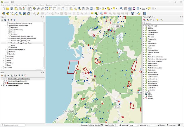
Explore the contents of the downloaded data by right clicking a layer and then choosing Open Attribute Table. Double clicking on the line number to the left zooms in on the object on the map. Save your project from time to time. Now that we have explored the data, it is time to check whether our sites are exposed to natural hazards.

4. Download pluvial hazard data from the County Administrative Boards

The County Administrative Boards are the main data provider for pluvial (cloudburst) data covering larger areas. We can obtain hazard data from the County Administrative Boards geodata catalogue. The data is provided per county based on a county code. The following table lists all counties and their respective codes. Go the geodata catalogue and look for a county of interest. For Gotland, use the search string ‘LSTI Lågpunktskartering’. There are other models than depression mapping with varying water levels both in raster and vector format. The methodology presented here is hence not one-to-one transferable to other datasets. This also affects the searchstring. If unsure, just search by county code and browse through the files.

You should have found 3 data layers as shown in Figure 2. We are interested in the inundation area in case of a cloudburst event. The Atom symbol under Länkar indicates that the dataset is downloadable. Open the files and read about the metadata. Then download the two files LstI Lågpunktskartering Isolerade områden lägre än 0,2 meter and LstI Lågpunktskartering Isolerade områden lägre än 1 meter.

5. Visualize the inundation layers in QGIS

Extract the files, go back to your QGIS project and browse to the folder with the new datasets. Identify the .shp extensions in the geopackage and drag them on the map just above the OpenStreetMap background map. Place the …1M inundation depth layer above the 02M layer since the extent is smaller (fewer areas will be inundated up to one meter in depth than 20 cm). Adjust the symbology, e.g. by changing the colour to shades of blue, removing the outline (stroke style) and making the layer partly transparent (use the opacity slider). The result could look like the example in Figure 3.
 

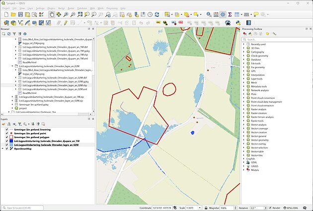
6. Explore and quantify exposed cultural heritage objects

Based on visual interpretation, it becomes clear to what extent cultural heritage sites are exposed to pluvial flood hazards. There are several ways of quantifying the degree of exposure across all datasets. In this tutorial, we will showcase how we can summarize the degree of exposure using spatial operations and recording the data in the attribute table?
The attribute table displays information on features of a selected layer. Each row in the table represents a feature (with or without geometry), and each column contains a particular piece of information about the feature. Features in the table can be searched, selected, moved or even edited. We will first add fields to the attribute table that will contain information about exposure to floods.
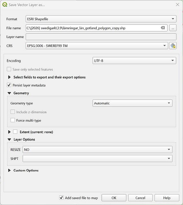
Prior to that, we will create editable shapefile copies of the three layers lämningar_län_gotland_polygon; lämningar_län_gotland_linestring and lämningar_län_gotland_point. Right-click each of the layers and select Export > Save Feature As…. Choose ESRI shapefile and save it at an appropriate location as shown in Figure 4. Don’t change any of the other settings. Adjust the symbology of the new layers and remove the original ones.
 

6.1 Adding fields
Open the attribute table for the new shapefiles and add the following two new fields to the respective layers according to Table 2. First make the table editable by Toggeling edit mode ( ). Then click the New field symbol ( ).
 

After having created the new layers, click the Toggeling edit mode again ( ) to deactivate modifying the table. If prompted, save your edits.

6.2 Fixing geometries and indexing
The geometries of spatial layers sometimes suffer from inconsistencies, e.g. polygons that do not exactly close or line features that have dangles or are too short. To ensure that spatial operations run smoothly, we first fix the geometries of all layers. This is a general recommendation when working with geodata from different sources. In the Processing Toolbox to the right-hand side of the QGIS GUI search for ‘fix geometry’. Choose the function Fix geometries under Vector geometry. Fix all geometries and save the vector files with the suffix ‘_fixed’.

To improve performance and drastically reduce computation time, we will add a spatial index to the features in the vector layers. In the Processing Toolbox, search for Create spatial index (located under the Vector general section). Create an index for all five data layers with fixed geometries.

6.3 Analysing and quantifying exposure to floods
The Flood_1m and Flood_02m fields will contain the binary information of whether a feature in the list is affected by the 0.2m and 1m inundation layers [yes] or not [no]. To determine whether a point feature will be flooded in case of a cloudburst event or not, we will perform queries based on spatial location. We run the Select by location algorithm ( ) using SQL. We first choose the point layer lämningar_län_gotland_point_copy_fixed as input (Select features from). We choose the spatial relationship are within under (Where the features) and finally, we select the layer to be compared to the layer containing the inundated surfaces Lsti.lagpunktskartering_Isolerade_Omraden_djupare_an_1Mfixed (By comparing to the features from).

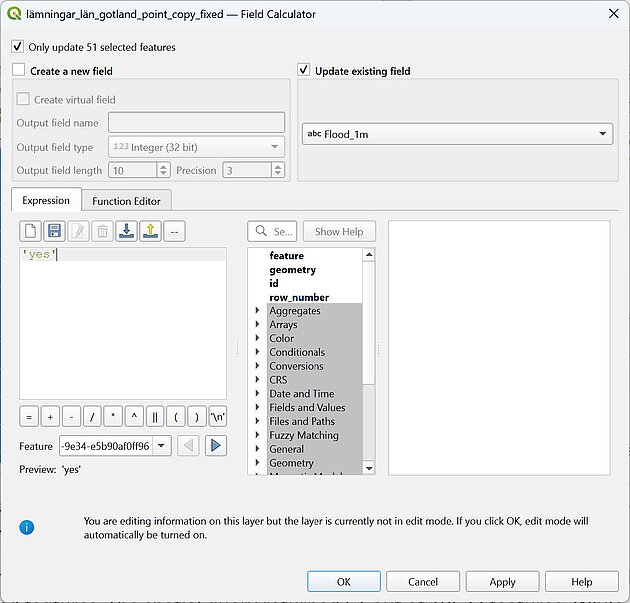
After the operation is complete, open the attribute table of lämningar_län_gotland_point_copy_fixed. In the lower left corner, choose Show selected features. The spatial query returned 51 out of 19,532 features. While having the points selected, open the Field Calculator ( ). Choose Update existing field and write ‘yes’ in the Expression field and click Apply and OK as exemplified in Figure 5. If the operation succeeded, you should now see ‘yes’ in the attribute table for 51 features under the Flood_1m column.

Perform the same spatial query with the other flood layer Lsti.Lagpunktskartering_Isolerade_Omraden_lagre_an_02Mfixed and update the attribute table accordingly. This query should have returned 555 features.

Now let’s have a look at line features. In the Select by location function, we need to choose another spatial relationship than are within because line features might only be partially covered by the inundation layer. We choose to intersect instead. Running the algorithm on the Lsti.Lagpunktskartering_Isolerade_Omraden_lagre_an_1Mfixed layer returns 54 features and on the Lsti.Lagpunktskartering_Isolerade_Omraden_lagre_an_02Mfixed layer 1,103features. Update the attribute table accordingly.

The last layer is a polygon layer. Here we again need to choose a different spatial relationship. In this case, overlap is the right choice. If you would like to have more information on the

different spatial relationships, consult the Help section in the Select by location dialogue or the documentation. Performing the operation results in 153 features for the Lsti.Lagpunktskartering_Isolerade_Omraden_lagre_an_1Mfixed layer and in 1,992 features for the Lsti.Lagpunktskartering_Isolerade_Omraden_lagre_an_02Mfixed layer.

To calculate the inundated area, we use the Overlap analysis under Vector analysis from the Processing Toolbox. This algorithm calculates the area and percentage cover by which features from an input layer are overlapped by features from a selection of overlay layers. New attributes are added to the output layer reporting the total area of overlap and percentage of the input feature overlapped by each of the selected overlay layers. Run the algorithm with the settings below. As Overlay layers, choose the inundation surfaces.
 

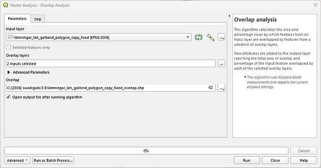
Open the attribute table of the new overlay layer. Four new columns have been added at the end (Lsti.lagpu; Lsti.lag_1; Lsti.lag_2 and Lsti.lag_3). Lsti.lagpu contains the overlapping area from the 1m flood layer and Lsti.lag_2 the area from the 20cm flood layer. Activate Toggeling edit mode ( ) and remove the fields Lsti.lag_1 and Lsti.lag_3 containing the overlap percentage with Delete field ( ).

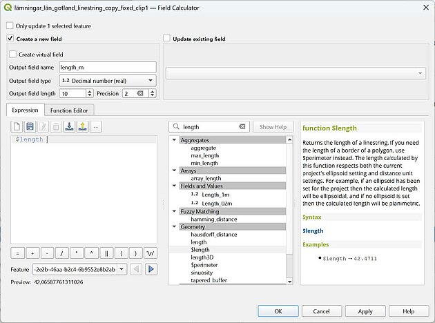
To calculate the length of potentially flooded line features, we first clip the line features to isolate the inundated part. Use the Clip function under Vector overlay. This algorithm clips a vector layer using the features of an additional polygon layer. Only the parts of the features in the Input layer that fall within the polygons of the Overlay layer will be added to the resulting layer. The attributes of the features are not modified, although properties such as area or length of the features will be modified by the clipping operation. As input layer, choose the lämningar_län_gotland_linestring_copy_fixed layer and as Overlay layer, both flood surfaces (first one, then the other) and save the output accordingly as a shapefile. The clipped layer consists of 54 line features for the 1 m depth scenario and 1,103 features for the 20 cm

inundation layer. To calculate the length of the line segments, use the Field Calculator as you did before and run the calculator with the settings as shown in Figure 7. Close the attribute table and when prompted make sure you save the results and toggle off editing mode.